Support Vector Machine
In this module, we introduce the Support Vector Machine (SVM) algorithm, a powerful, but simple supervised learning approach to predicting data. For classification tasks, the SVM algorithm attempts to divide data in the feature space into distinct categories. By default, this division is performed by constructing hyperplanes that optimally divide the data. For regression, the hyperplanes are constructed to map the distribution of data. In both cases, these hyperplanes map linear structures in a non-probabilistic manner. By employing a kernel trick, however, we can transform non-linear data sets into linear ones, thus enabling SVM to be applied to non-linear problems.
SVMs are powerful algorithms that have gained widespread popularity. This is due partly to the fact that they are effective in high dimensional feature spaces, including those problems where the number of features is similar to or slightly exceeds the number of instances. They can also be memory efficient since only the support vectors are needed to compute the hyperplanes. Finally, by using different kernels, SVM can be applied to a wide range of learning tasks. On the other hand, these models are black boxes, and it can be difficult to explain how they operate, especially on new instances. They do not, by default, provide probability estimates, since the hyperplane is constructed to cleanly divide the training data.
In this module, we first explore the basic formalism of the SVM algorithm, including the construction of hyperplanes and the kernel trick, which enables SVM to be applied to non-linear problems. Next, we explore the application of SVM to classification problems, which is known as support vector classification, or SVC. To introduce this topic, we will once again use the Iris data to construct an SVC estimator, explore the resulting performance and decision surface, before looking at the effect of different hyperparameter values. Next, we will switch to a more complex data set, the adult data demonstrated in the Introduction to Decision Tree module, with which we will explore unbalanced classes and more advanced classification performance metrics such as the ROC, AUC, and Lift curve. Finally, we will apply SVM to regression problems, which is known as support vector regression. For this we will use the automobile miles per gallon regression task first presented in the Introduction to Decision Tree module.
Formalism
As was the case with the decision tree, one of the simplest machine learning algorithms to understand and employ is the support vector machine. For classification tasks, this algorithm simply divides the data with hyperplanes into the resulting classes, while for regression, the hyperplanes form a predictive model of the underlying data. These hyperplanes, by default, produce a linear classifier (or regressor) since they are restricted to be linear in the features. However, unlike a decision tree, SVM produces a black box model; we can’t examine the model, especially in higher dimensions, to understand why specific predictions are made. In order to construct the optimal set of hyperplanes, SVM assumes the features are normalized and can be compared equally. Thus, for proper use of an SVM on a data set, we must normalize the features.
Given a set of data with \(n\) features, we can construct many different hyperplanes that divide the data. The SVM algorithm selects the optimal hyperplane by finding the one that produces the largest separation, which is known as the margin, between the data. The hyperplane that accomplishes this goal is known as the maximum-margin hyperplane. For high dimensional data, a set of hyperplanes is constructed, which accomplishes this same task. In cases where the data cannot be cleanly separated, many SVM implementations map the data set into a higher dimensional space by using a kernel function, where the data are linearly separated and construct a set of optimal hyperplanes in this space. This process can also be used to transform a non-linear feature space into a linear (or approximately linear) space where traditional SVM can be applied.
In the rest of this section, we demonstrate the construction of hyperplanes by using the Iris data set. To simplify the visualization of these data and the resulting hyperplanes, we use only two dimensions. Since SVM, by default, provides a linear classification, these hyperplanes will generate linear divisions between classes. After this, we demonstrate how a kernel can be employed to transform a non-linear problem into a linear classification task.
Hyperplanes
To demonstrate how hyperplanes can divide data, we will use the standard Iris classification data set. We first use our helper functions to load the Iris data and subdivide into training and testing. We normalize the data by using the training function. Next, we select only two dimensions: Sepal Width and Petal Width, to use in our subsequent analysis to enable easier visualization of the training data, test data, and hyperplanes.
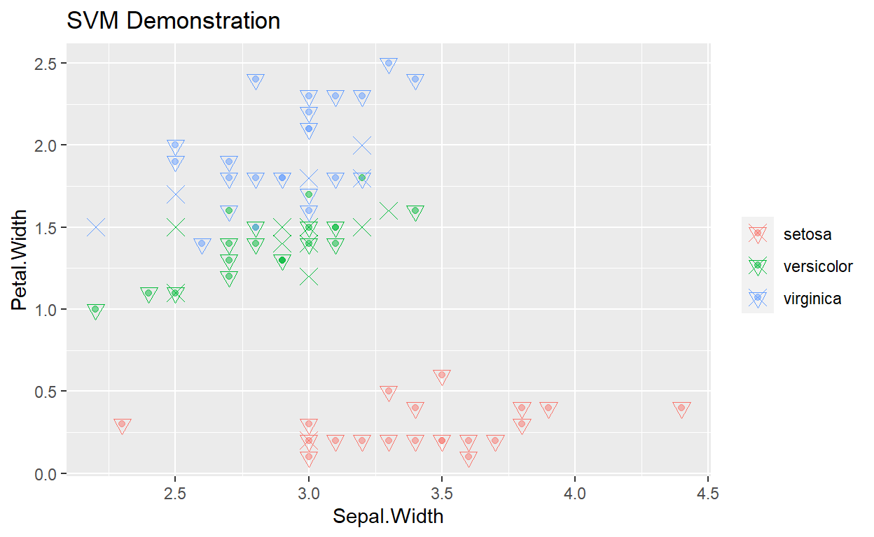
There Code chunk uses the training data to generate an SVC (don’t worry about the details of doing this right now, they are introduced in the next section). Next, we make a scatter plot of the training data, colored by their label, and display test data with a different symbol. Next, we generate a grid of points through this space and apply the predetermined SVC to generate decisions over this grid (note, this is similar to how we construct decisions surfaces for classification tasks). Finally, the algorithm generates a separate hyperplane to divide between each set of classes. The support vectors used to compute these hyperplanes from the training data.
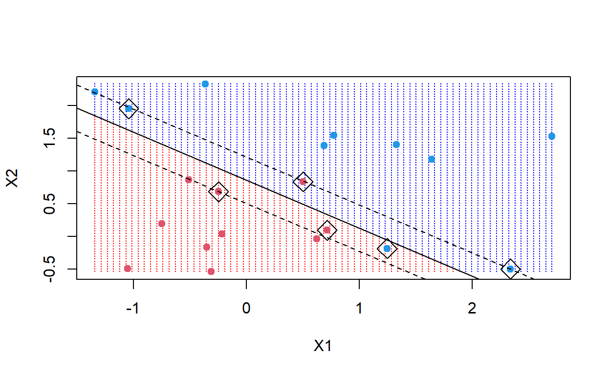
The hyperplanes shown in the plot are denoted by the solid gray line. We also plot the confidence interval (or upper and lower one-sigma standard deviations) for these hyperplanes, the upper boundary as a blue dashed line, and the lower boundary as a red dashed line. The confidence interval in this case provides an estimate for the uncertainty in the location of the true hyperplane given these training data.
The support are those training data that are used to finalize the selection of the best hyperplane. The training data that anchor the support vectors are enclosed in diamonds. The vector extends from these points to the hyperplane (forming a right angle to the hyperplane). The margin for each support vector is the distance from the support to the hyperplane (or the length of the support vector). It is the combinations of these distances that we seek to minimize when we compute the best hyperplane.
library(caret)
library(tidyverse)
#set the seed :)
set.seed(1)
#get our samples
#using the iris data
#lets split the data 60/40

trainIndex <- createDataPartition(iris$Species, p = .6, list = FALSE, times = 1)

#look at the first few
#head(trainIndex)

#grab the data
SVMTrain <- iris[ trainIndex,]
SVMTest  <- iris[-trainIndex,]


iris_SVM <- train(
  form = factor(Species) ~ .,
  data = SVMTrain,
  #here we add classProbs because we want probs
  trControl = trainControl(method = "cv", number = 10,
                           classProbs =  TRUE),
  method = "svmLinear",
  preProcess = c("center", "scale"),
  tuneLength = 10)

iris_SVM
Support Vector Machines with Linear Kernel

90 samples
 4 predictor
 3 classes: 'setosa', 'versicolor', 'virginica'

Pre-processing: centered (4), scaled (4)
Resampling: Cross-Validated (10 fold)
Summary of sample sizes: 81, 81, 81, 81, 81, 81, ...
Resampling results:

  Accuracy   Kappa
  0.9666667  0.95

Tuning parameter 'C' was held constant at a value of 1summary(iris_SVM)
Length  Class   Mode
1 ksvm S4 svm_Pred<-predict(iris_SVM,SVMTest,type="prob")
knitr::kable(svm_Pred)%>%
kableExtra::kable_styling("striped")%>%
kableExtra::scroll_box(width = "100%",height="300px")
| setosa | versicolor | virginica |
|---|---|---|
| 0.9119900 | 0.0667780 | 0.0212320 |
| 0.9765986 | 0.0122676 | 0.0111338 |
| 0.9610351 | 0.0239773 | 0.0149876 |
| 0.9765749 | 0.0119585 | 0.0114666 |
| 0.9313294 | 0.0509379 | 0.0177327 |
| 0.9897054 | 0.0027805 | 0.0075140 |
| 0.9796212 | 0.0090689 | 0.0113100 |
| 0.9699558 | 0.0153175 | 0.0147267 |
| 0.8910858 | 0.0775756 | 0.0313386 |
| 0.9664487 | 0.0196413 | 0.0139099 |
| 0.9408605 | 0.0403384 | 0.0188011 |
| 0.9313729 | 0.0459459 | 0.0226812 |
| 0.9252151 | 0.0544007 | 0.0203842 |
| 0.9677491 | 0.0192658 | 0.0129851 |
| 0.9816657 | 0.0092066 | 0.0091277 |
| 0.6082704 | 0.3585779 | 0.0331517 |
| 0.9227571 | 0.0492752 | 0.0279676 |
| 0.9650908 | 0.0172381 | 0.0176711 |
| 0.8958313 | 0.0797438 | 0.0244249 |
| 0.9546095 | 0.0296492 | 0.0157413 |
| 0.0148830 | 0.8755405 | 0.1095765 |
| 0.0105902 | 0.8928634 | 0.0965464 |
| 0.0145113 | 0.9657228 | 0.0197658 |
| 0.0240048 | 0.9340854 | 0.0419098 |
| 0.0076557 | 0.9901118 | 0.0022325 |
| 0.0549154 | 0.9289241 | 0.0161605 |
| 0.0230323 | 0.9559715 | 0.0209962 |
| 0.0205240 | 0.9731425 | 0.0063335 |
| 0.0420572 | 0.2132697 | 0.7446731 |
| 0.0182047 | 0.9581886 | 0.0236067 |
| 0.0081877 | 0.9374497 | 0.0543626 |
| 0.0206738 | 0.4701043 | 0.5092219 |
| 0.0172608 | 0.9773076 | 0.0054315 |
| 0.0266853 | 0.9644647 | 0.0088500 |
| 0.0223888 | 0.3318986 | 0.6457126 |
| 0.0363084 | 0.7313350 | 0.2323566 |
| 0.0525471 | 0.7533945 | 0.1940585 |
| 0.0173036 | 0.8980045 | 0.0846920 |
| 0.0188206 | 0.9541401 | 0.0270393 |
| 0.0316689 | 0.9438493 | 0.0244817 |
| 0.0089516 | 0.0056648 | 0.9853836 |
| 0.0189757 | 0.0420633 | 0.9389610 |
| 0.0091081 | 0.0016704 | 0.9892215 |
| 0.0050442 | 0.0015931 | 0.9933626 |
| 0.0098296 | 0.0232422 | 0.9669282 |
| 0.0147971 | 0.0452636 | 0.9399392 |
| 0.0140854 | 0.0175944 | 0.9683202 |
| 0.0091980 | 0.0009526 | 0.9898494 |
| 0.0195324 | 0.2140618 | 0.7664057 |
| 0.0230968 | 0.2482140 | 0.7286892 |
| 0.0168276 | 0.2930305 | 0.6901419 |
| 0.0173931 | 0.6274968 | 0.3551101 |
| 0.0182957 | 0.3913999 | 0.5903043 |
| 0.0048002 | 0.0015258 | 0.9936740 |
| 0.0123775 | 0.0008602 | 0.9867622 |
| 0.0246667 | 0.0682397 | 0.9070936 |
| 0.0125091 | 0.0088514 | 0.9786395 |
| 0.0085294 | 0.0010148 | 0.9904558 |
| 0.0078415 | 0.0004231 | 0.9917355 |
| 0.0139480 | 0.0789715 | 0.9070805 |
svmtestpred<-cbind(svm_Pred,SVMTest)

svmtestpred<-svmtestpred%>%
  mutate(prediction=if_else(setosa>versicolor & setosa>virginica,"setosa",
                            if_else(versicolor>setosa & versicolor>virginica, "versicolor",
                                    if_else(virginica>setosa & virginica>versicolor,"virginica", "PROBLEM"))))

table(svmtestpred$prediction)
    setosa versicolor  virginica
20 18 22 confusionMatrix(factor(svmtestpred$prediction),factor(svmtestpred$Species))
Confusion Matrix and Statistics

            Reference
Prediction   setosa versicolor virginica
  setosa         20          0         0
  versicolor      0         17         1
  virginica       0          3        19

Overall Statistics

               Accuracy : 0.9333
                 95% CI : (0.838, 0.9815)
    No Information Rate : 0.3333
    P-Value [Acc > NIR] : < 2.2e-16

                  Kappa : 0.9

 Mcnemar's Test P-Value : NA

Statistics by Class:

                     Class: setosa Class: versicolor Class: virginica
Sensitivity                 1.0000            0.8500           0.9500
Specificity                 1.0000            0.9750           0.9250
Pos Pred Value              1.0000            0.9444           0.8636
Neg Pred Value              1.0000            0.9286           0.9737
Prevalence                  0.3333            0.3333           0.3333
Detection Rate              0.3333            0.2833           0.3167
Detection Prevalence        0.3333            0.3000           0.3667
Balanced Accuracy 1.0000 0.9125 0.9375supportvectors<-SVMTrain[iris_SVM$finalModel@SVindex,]
ggplot(data=SVMTest, mapping = aes(x=Sepal.Width,y=Petal.Width,color=Species))+
geom_point(alpha=0.5)+
geom_point(data=svmtestpred, mapping = aes(x=Sepal.Width,y=Petal.Width, color=prediction),shape=6,size=3)+
geom_point(data=supportvectors, mapping = aes(x=Sepal.Width,y=Petal.Width),shape=4,size=4)+
theme(legend.title = element_blank())+ggtitle("SVM Demonstration")
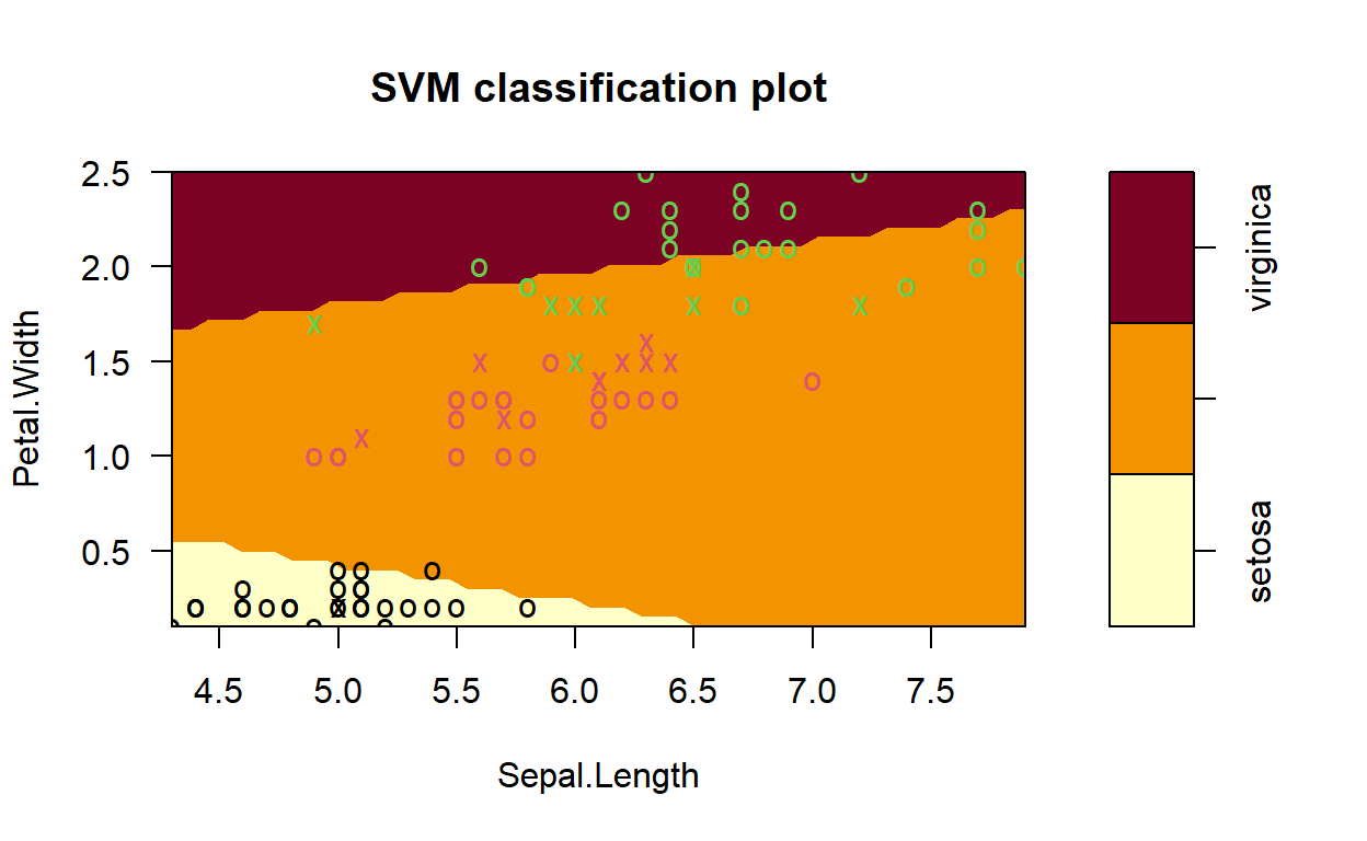
svmfit = e1071::svm(Species~., data = SVMTrain, kernel = "linear", cost = 1, scale = TRUE)

# Plot Results
plot(svmfit, SVMTrain, Petal.Width ~ Sepal.Length,
     slice = list(Sepal.Width = 3, Petal.Length = 4))
Call:
svm(formula = y ~ ., data = dat, kernel = "linear", cost = 10,
    scale = FALSE)


Parameters:
   SVM-Type:  C-classification
 SVM-Kernel:  linear
       cost:  10

Number of Support Vectors:  6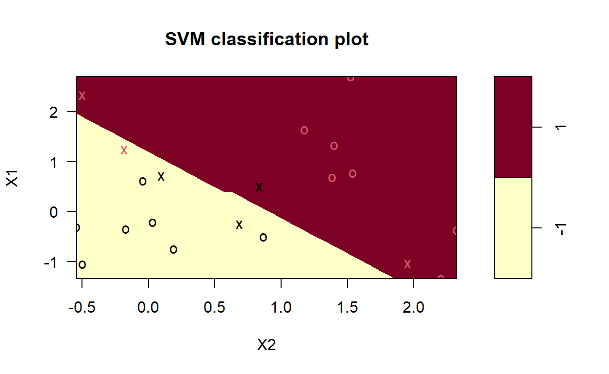
           X1         X2
1  -1.3406379 -0.5400074
2  -1.2859572 -0.5400074
3  -1.2312766 -0.5400074
4  -1.1765959 -0.5400074
5  -1.1219153 -0.5400074
6  -1.0672346 -0.5400074
7  -1.0125540 -0.5400074
8  -0.9578733 -0.5400074
9  -0.9031927 -0.5400074
10 -0.8485120 -0.5400074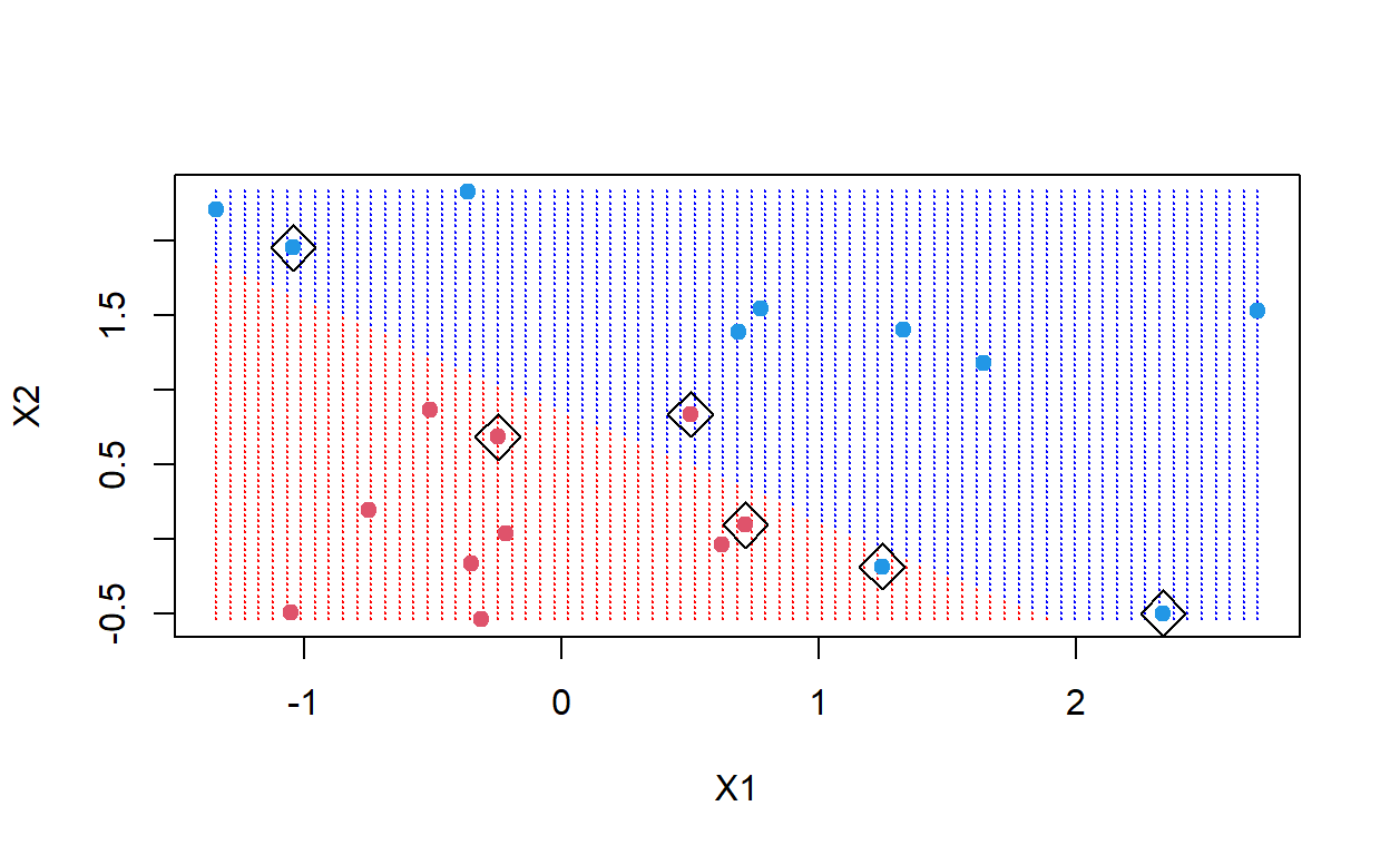
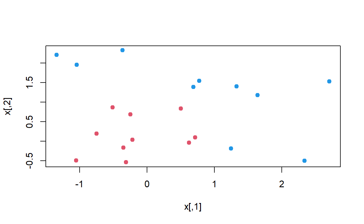
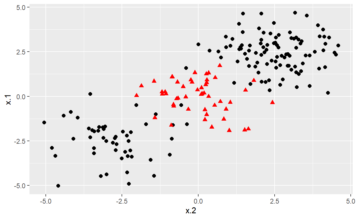
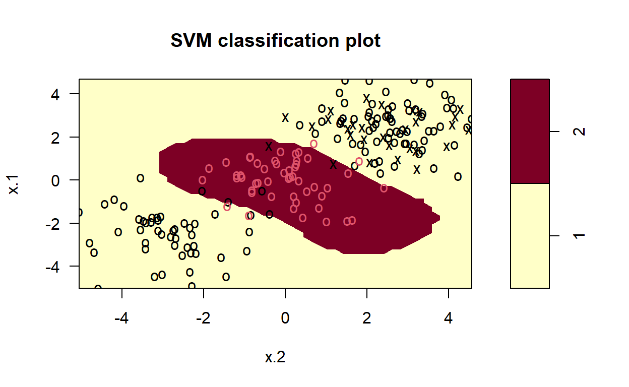
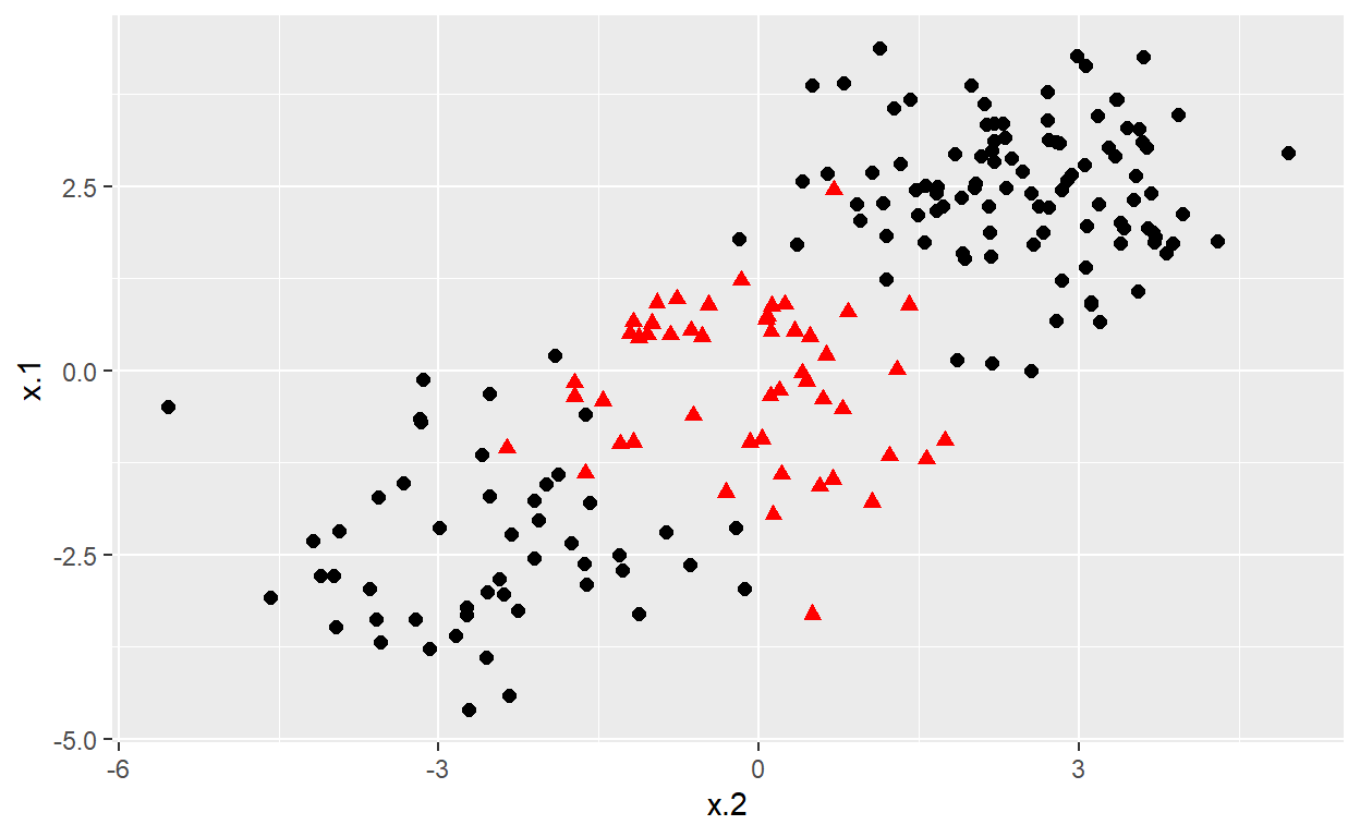
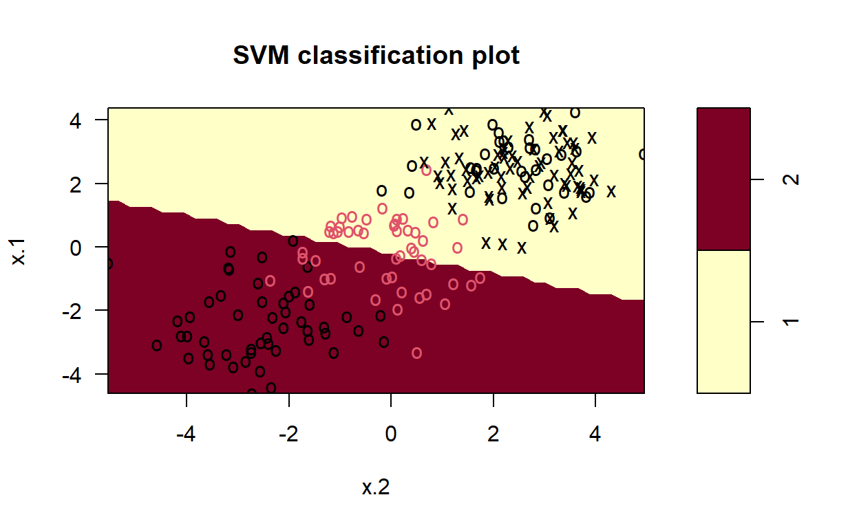
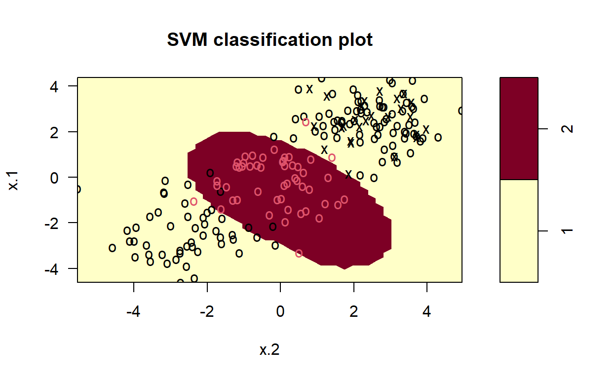
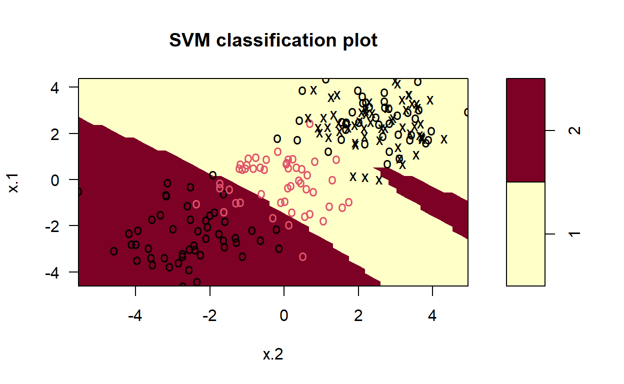
# construct larger random data set
x <- matrix(rnorm(200*2), ncol = 2)
x[1:100,] <- x[1:100,] + 2.5
x[101:150,] <- x[101:150,] - 2.5
y <- c(rep(1,150), rep(2,50))
dat <- data.frame(x=x,y=as.factor(y))

# Plot data
ggplot(data = dat, aes(x = x.2, y = x.1, color = y, shape = y)) +
  geom_point(size = 2) +
  scale_color_manual(values=c("#000000", "#FF0000")) +
  theme(legend.position = "none")
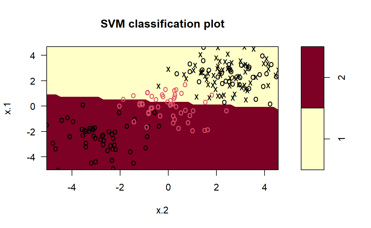
library(e1071)

# set pseudorandom number generator
set.seed(123)
# sample training data and fit model
train <- base::sample(200,100, replace = FALSE)
svmfit <- svm(y~., data = dat[train,],  kernel = "linear", cost = 10, scale = FALSE)
# plot classifier
plot(svmfit, dat)
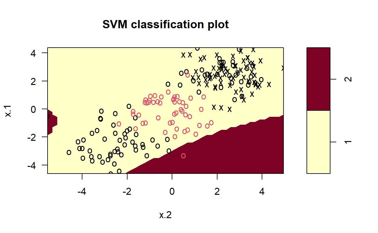
Non-Linear Kernels
In many real-world cases, the data of interest are non-linear. In these cases, we can still successfully employ SVM by transforming the data into a space where the data are linearly separated. This process is known as the kernel trick, since we employ a kernel function to perform the mapping.
svmfit <- svm(y~., data = dat[train,], kernel = "radial", gamma = 1, cost = 1)
# plot classifier
plot(svmfit, dat)
Exercise 1
Use the first code chunk with the iris data.
Change the training to testing split size, for example change from a 60%:40% to a 75%:25%, and to a 50%:50%. Compare the results to the 60/40.
Change the Kernel…use svmPoly for the method.
method = "svmLinear",tomethod = "svmPoly",compare the linear results with the polynomial results.
SVM: Hyperparameters1
Perhaps the most important hyperparameter for SVC is the kernel hyperparameter, which specifies the type of transformation that should be applied to the training data to determine the optimal set of hyperplanes. In the previous example, we computed and displayed the decision surface for a linear kernel. n the following Code chunks, we compute and display decision surfaces for SVCs that employ different kernel functions: linear, polynomial, radial, and sigmoid. By doing this, the resulting figures demonstrate how these different kernels affect the classification.
Note how the resulting decisions surfaces are no longer dominated by the linear divisions. Each of the last three decision surfaces have curved hyperplanes in the original space, since they transform the original data by using non-linear functions. Radial peforms the best.
Linear
Radial
Sigmoid
Polynomial
Exercise 2
- Look back at the SVM’s run for the iris data. What where the hyperparameters chose for the Linear kernel, Radial kernel, and the Polynomial kernel? What are each of these hyperparameters?
Classification: Adult Data
We now transition to a more complex data set, the adult data from the UCI machine learning repository. These data are fully documented online at the UCI website.
# install.packages("devtools")
# devtools::install_github("tyluRp/ucimlr")

adult<-ucimlr::adult


knitr::kable(head(adult,100))%>%
  kableExtra::kable_styling("striped")%>%
  kableExtra::scroll_box(width = "100%",height="300px")
| age | workclass | fnlwgt | education | education_num | marital_status | occupation | relationship | race | sex | capital_gain | capital_loss | hours_per_week | native_country | income |
|---|---|---|---|---|---|---|---|---|---|---|---|---|---|---|
| 50 | Self-emp-not-inc | 83311 | Bachelors | 13 | Married-civ-spouse | Exec-managerial | Husband | White | Male | 0 | 0 | 13 | United-States | <=50K |
| 38 | Private | 215646 | HS-grad | 9 | Divorced | Handlers-cleaners | Not-in-family | White | Male | 0 | 0 | 40 | United-States | <=50K |
| 53 | Private | 234721 | 11th | 7 | Married-civ-spouse | Handlers-cleaners | Husband | Black | Male | 0 | 0 | 40 | United-States | <=50K |
| 28 | Private | 338409 | Bachelors | 13 | Married-civ-spouse | Prof-specialty | Wife | Black | Female | 0 | 0 | 40 | Cuba | <=50K |
| 37 | Private | 284582 | Masters | 14 | Married-civ-spouse | Exec-managerial | Wife | White | Female | 0 | 0 | 40 | United-States | <=50K |
| 49 | Private | 160187 | 9th | 5 | Married-spouse-absent | Other-service | Not-in-family | Black | Female | 0 | 0 | 16 | Jamaica | <=50K |
| 52 | Self-emp-not-inc | 209642 | HS-grad | 9 | Married-civ-spouse | Exec-managerial | Husband | White | Male | 0 | 0 | 45 | United-States | >50K |
| 31 | Private | 45781 | Masters | 14 | Never-married | Prof-specialty | Not-in-family | White | Female | 14084 | 0 | 50 | United-States | >50K |
| 42 | Private | 159449 | Bachelors | 13 | Married-civ-spouse | Exec-managerial | Husband | White | Male | 5178 | 0 | 40 | United-States | >50K |
| 37 | Private | 280464 | Some-college | 10 | Married-civ-spouse | Exec-managerial | Husband | Black | Male | 0 | 0 | 80 | United-States | >50K |
| 30 | State-gov | 141297 | Bachelors | 13 | Married-civ-spouse | Prof-specialty | Husband | Asian-Pac-Islander | Male | 0 | 0 | 40 | India | >50K |
| 23 | Private | 122272 | Bachelors | 13 | Never-married | Adm-clerical | Own-child | White | Female | 0 | 0 | 30 | United-States | <=50K |
| 32 | Private | 205019 | Assoc-acdm | 12 | Never-married | Sales | Not-in-family | Black | Male | 0 | 0 | 50 | United-States | <=50K |
| 40 | Private | 121772 | Assoc-voc | 11 | Married-civ-spouse | Craft-repair | Husband | Asian-Pac-Islander | Male | 0 | 0 | 40 | NA | >50K |
| 34 | Private | 245487 | 7th-8th | 4 | Married-civ-spouse | Transport-moving | Husband | Amer-Indian-Eskimo | Male | 0 | 0 | 45 | Mexico | <=50K |
| 25 | Self-emp-not-inc | 176756 | HS-grad | 9 | Never-married | Farming-fishing | Own-child | White | Male | 0 | 0 | 35 | United-States | <=50K |
| 32 | Private | 186824 | HS-grad | 9 | Never-married | Machine-op-inspct | Unmarried | White | Male | 0 | 0 | 40 | United-States | <=50K |
| 38 | Private | 28887 | 11th | 7 | Married-civ-spouse | Sales | Husband | White | Male | 0 | 0 | 50 | United-States | <=50K |
| 43 | Self-emp-not-inc | 292175 | Masters | 14 | Divorced | Exec-managerial | Unmarried | White | Female | 0 | 0 | 45 | United-States | >50K |
| 40 | Private | 193524 | Doctorate | 16 | Married-civ-spouse | Prof-specialty | Husband | White | Male | 0 | 0 | 60 | United-States | >50K |
| 54 | Private | 302146 | HS-grad | 9 | Separated | Other-service | Unmarried | Black | Female | 0 | 0 | 20 | United-States | <=50K |
| 35 | Federal-gov | 76845 | 9th | 5 | Married-civ-spouse | Farming-fishing | Husband | Black | Male | 0 | 0 | 40 | United-States | <=50K |
| 43 | Private | 117037 | 11th | 7 | Married-civ-spouse | Transport-moving | Husband | White | Male | 0 | 2042 | 40 | United-States | <=50K |
| 59 | Private | 109015 | HS-grad | 9 | Divorced | Tech-support | Unmarried | White | Female | 0 | 0 | 40 | United-States | <=50K |
| 56 | Local-gov | 216851 | Bachelors | 13 | Married-civ-spouse | Tech-support | Husband | White | Male | 0 | 0 | 40 | United-States | >50K |
| 19 | Private | 168294 | HS-grad | 9 | Never-married | Craft-repair | Own-child | White | Male | 0 | 0 | 40 | United-States | <=50K |
| 54 | NA | 180211 | Some-college | 10 | Married-civ-spouse | NA | Husband | Asian-Pac-Islander | Male | 0 | 0 | 60 | South | >50K |
| 39 | Private | 367260 | HS-grad | 9 | Divorced | Exec-managerial | Not-in-family | White | Male | 0 | 0 | 80 | United-States | <=50K |
| 49 | Private | 193366 | HS-grad | 9 | Married-civ-spouse | Craft-repair | Husband | White | Male | 0 | 0 | 40 | United-States | <=50K |
| 23 | Local-gov | 190709 | Assoc-acdm | 12 | Never-married | Protective-serv | Not-in-family | White | Male | 0 | 0 | 52 | United-States | <=50K |
| 20 | Private | 266015 | Some-college | 10 | Never-married | Sales | Own-child | Black | Male | 0 | 0 | 44 | United-States | <=50K |
| 45 | Private | 386940 | Bachelors | 13 | Divorced | Exec-managerial | Own-child | White | Male | 0 | 1408 | 40 | United-States | <=50K |
| 30 | Federal-gov | 59951 | Some-college | 10 | Married-civ-spouse | Adm-clerical | Own-child | White | Male | 0 | 0 | 40 | United-States | <=50K |
| 22 | State-gov | 311512 | Some-college | 10 | Married-civ-spouse | Other-service | Husband | Black | Male | 0 | 0 | 15 | United-States | <=50K |
| 48 | Private | 242406 | 11th | 7 | Never-married | Machine-op-inspct | Unmarried | White | Male | 0 | 0 | 40 | Puerto-Rico | <=50K |
| 21 | Private | 197200 | Some-college | 10 | Never-married | Machine-op-inspct | Own-child | White | Male | 0 | 0 | 40 | United-States | <=50K |
| 19 | Private | 544091 | HS-grad | 9 | Married-AF-spouse | Adm-clerical | Wife | White | Female | 0 | 0 | 25 | United-States | <=50K |
| 31 | Private | 84154 | Some-college | 10 | Married-civ-spouse | Sales | Husband | White | Male | 0 | 0 | 38 | NA | >50K |
| 48 | Self-emp-not-inc | 265477 | Assoc-acdm | 12 | Married-civ-spouse | Prof-specialty | Husband | White | Male | 0 | 0 | 40 | United-States | <=50K |
| 31 | Private | 507875 | 9th | 5 | Married-civ-spouse | Machine-op-inspct | Husband | White | Male | 0 | 0 | 43 | United-States | <=50K |
| 53 | Self-emp-not-inc | 88506 | Bachelors | 13 | Married-civ-spouse | Prof-specialty | Husband | White | Male | 0 | 0 | 40 | United-States | <=50K |
| 24 | Private | 172987 | Bachelors | 13 | Married-civ-spouse | Tech-support | Husband | White | Male | 0 | 0 | 50 | United-States | <=50K |
| 49 | Private | 94638 | HS-grad | 9 | Separated | Adm-clerical | Unmarried | White | Female | 0 | 0 | 40 | United-States | <=50K |
| 25 | Private | 289980 | HS-grad | 9 | Never-married | Handlers-cleaners | Not-in-family | White | Male | 0 | 0 | 35 | United-States | <=50K |
| 57 | Federal-gov | 337895 | Bachelors | 13 | Married-civ-spouse | Prof-specialty | Husband | Black | Male | 0 | 0 | 40 | United-States | >50K |
| 53 | Private | 144361 | HS-grad | 9 | Married-civ-spouse | Machine-op-inspct | Husband | White | Male | 0 | 0 | 38 | United-States | <=50K |
| 44 | Private | 128354 | Masters | 14 | Divorced | Exec-managerial | Unmarried | White | Female | 0 | 0 | 40 | United-States | <=50K |
| 41 | State-gov | 101603 | Assoc-voc | 11 | Married-civ-spouse | Craft-repair | Husband | White | Male | 0 | 0 | 40 | United-States | <=50K |
| 29 | Private | 271466 | Assoc-voc | 11 | Never-married | Prof-specialty | Not-in-family | White | Male | 0 | 0 | 43 | United-States | <=50K |
| 25 | Private | 32275 | Some-college | 10 | Married-civ-spouse | Exec-managerial | Wife | Other | Female | 0 | 0 | 40 | United-States | <=50K |
| 18 | Private | 226956 | HS-grad | 9 | Never-married | Other-service | Own-child | White | Female | 0 | 0 | 30 | NA | <=50K |
| 47 | Private | 51835 | Prof-school | 15 | Married-civ-spouse | Prof-specialty | Wife | White | Female | 0 | 1902 | 60 | Honduras | >50K |
| 50 | Federal-gov | 251585 | Bachelors | 13 | Divorced | Exec-managerial | Not-in-family | White | Male | 0 | 0 | 55 | United-States | >50K |
| 47 | Self-emp-inc | 109832 | HS-grad | 9 | Divorced | Exec-managerial | Not-in-family | White | Male | 0 | 0 | 60 | United-States | <=50K |
| 43 | Private | 237993 | Some-college | 10 | Married-civ-spouse | Tech-support | Husband | White | Male | 0 | 0 | 40 | United-States | >50K |
| 46 | Private | 216666 | 5th-6th | 3 | Married-civ-spouse | Machine-op-inspct | Husband | White | Male | 0 | 0 | 40 | Mexico | <=50K |
| 35 | Private | 56352 | Assoc-voc | 11 | Married-civ-spouse | Other-service | Husband | White | Male | 0 | 0 | 40 | Puerto-Rico | <=50K |
| 41 | Private | 147372 | HS-grad | 9 | Married-civ-spouse | Adm-clerical | Husband | White | Male | 0 | 0 | 48 | United-States | <=50K |
| 30 | Private | 188146 | HS-grad | 9 | Married-civ-spouse | Machine-op-inspct | Husband | White | Male | 5013 | 0 | 40 | United-States | <=50K |
| 30 | Private | 59496 | Bachelors | 13 | Married-civ-spouse | Sales | Husband | White | Male | 2407 | 0 | 40 | United-States | <=50K |
| 32 | NA | 293936 | 7th-8th | 4 | Married-spouse-absent | NA | Not-in-family | White | Male | 0 | 0 | 40 | NA | <=50K |
| 48 | Private | 149640 | HS-grad | 9 | Married-civ-spouse | Transport-moving | Husband | White | Male | 0 | 0 | 40 | United-States | <=50K |
| 42 | Private | 116632 | Doctorate | 16 | Married-civ-spouse | Prof-specialty | Husband | White | Male | 0 | 0 | 45 | United-States | >50K |
| 29 | Private | 105598 | Some-college | 10 | Divorced | Tech-support | Not-in-family | White | Male | 0 | 0 | 58 | United-States | <=50K |
| 36 | Private | 155537 | HS-grad | 9 | Married-civ-spouse | Craft-repair | Husband | White | Male | 0 | 0 | 40 | United-States | <=50K |
| 28 | Private | 183175 | Some-college | 10 | Divorced | Adm-clerical | Not-in-family | White | Female | 0 | 0 | 40 | United-States | <=50K |
| 53 | Private | 169846 | HS-grad | 9 | Married-civ-spouse | Adm-clerical | Wife | White | Female | 0 | 0 | 40 | United-States | >50K |
| 49 | Self-emp-inc | 191681 | Some-college | 10 | Married-civ-spouse | Exec-managerial | Husband | White | Male | 0 | 0 | 50 | United-States | >50K |
| 25 | NA | 200681 | Some-college | 10 | Never-married | NA | Own-child | White | Male | 0 | 0 | 40 | United-States | <=50K |
| 19 | Private | 101509 | Some-college | 10 | Never-married | Prof-specialty | Own-child | White | Male | 0 | 0 | 32 | United-States | <=50K |
| 31 | Private | 309974 | Bachelors | 13 | Separated | Sales | Own-child | Black | Female | 0 | 0 | 40 | United-States | <=50K |
| 29 | Self-emp-not-inc | 162298 | Bachelors | 13 | Married-civ-spouse | Sales | Husband | White | Male | 0 | 0 | 70 | United-States | >50K |
| 23 | Private | 211678 | Some-college | 10 | Never-married | Machine-op-inspct | Not-in-family | White | Male | 0 | 0 | 40 | United-States | <=50K |
| 79 | Private | 124744 | Some-college | 10 | Married-civ-spouse | Prof-specialty | Other-relative | White | Male | 0 | 0 | 20 | United-States | <=50K |
| 27 | Private | 213921 | HS-grad | 9 | Never-married | Other-service | Own-child | White | Male | 0 | 0 | 40 | Mexico | <=50K |
| 40 | Private | 32214 | Assoc-acdm | 12 | Married-civ-spouse | Adm-clerical | Husband | White | Male | 0 | 0 | 40 | United-States | <=50K |
| 67 | NA | 212759 | 10th | 6 | Married-civ-spouse | NA | Husband | White | Male | 0 | 0 | 2 | United-States | <=50K |
| 18 | Private | 309634 | 11th | 7 | Never-married | Other-service | Own-child | White | Female | 0 | 0 | 22 | United-States | <=50K |
| 31 | Local-gov | 125927 | 7th-8th | 4 | Married-civ-spouse | Farming-fishing | Husband | White | Male | 0 | 0 | 40 | United-States | <=50K |
| 18 | Private | 446839 | HS-grad | 9 | Never-married | Sales | Not-in-family | White | Male | 0 | 0 | 30 | United-States | <=50K |
| 52 | Private | 276515 | Bachelors | 13 | Married-civ-spouse | Other-service | Husband | White | Male | 0 | 0 | 40 | Cuba | <=50K |
| 46 | Private | 51618 | HS-grad | 9 | Married-civ-spouse | Other-service | Wife | White | Female | 0 | 0 | 40 | United-States | <=50K |
| 59 | Private | 159937 | HS-grad | 9 | Married-civ-spouse | Sales | Husband | White | Male | 0 | 0 | 48 | United-States | <=50K |
| 44 | Private | 343591 | HS-grad | 9 | Divorced | Craft-repair | Not-in-family | White | Female | 14344 | 0 | 40 | United-States | >50K |
| 53 | Private | 346253 | HS-grad | 9 | Divorced | Sales | Own-child | White | Female | 0 | 0 | 35 | United-States | <=50K |
| 49 | Local-gov | 268234 | HS-grad | 9 | Married-civ-spouse | Protective-serv | Husband | White | Male | 0 | 0 | 40 | United-States | >50K |
| 33 | Private | 202051 | Masters | 14 | Married-civ-spouse | Prof-specialty | Husband | White | Male | 0 | 0 | 50 | United-States | <=50K |
| 30 | Private | 54334 | 9th | 5 | Never-married | Sales | Not-in-family | White | Male | 0 | 0 | 40 | United-States | <=50K |
| 43 | Federal-gov | 410867 | Doctorate | 16 | Never-married | Prof-specialty | Not-in-family | White | Female | 0 | 0 | 50 | United-States | >50K |
| 57 | Private | 249977 | Assoc-voc | 11 | Married-civ-spouse | Prof-specialty | Husband | White | Male | 0 | 0 | 40 | United-States | <=50K |
| 37 | Private | 286730 | Some-college | 10 | Divorced | Craft-repair | Unmarried | White | Female | 0 | 0 | 40 | United-States | <=50K |
| 28 | Private | 212563 | Some-college | 10 | Divorced | Machine-op-inspct | Unmarried | Black | Female | 0 | 0 | 25 | United-States | <=50K |
| 30 | Private | 117747 | HS-grad | 9 | Married-civ-spouse | Sales | Wife | Asian-Pac-Islander | Female | 0 | 1573 | 35 | NA | <=50K |
| 34 | Local-gov | 226296 | Bachelors | 13 | Married-civ-spouse | Protective-serv | Husband | White | Male | 0 | 0 | 40 | United-States | >50K |
| 29 | Local-gov | 115585 | Some-college | 10 | Never-married | Handlers-cleaners | Not-in-family | White | Male | 0 | 0 | 50 | United-States | <=50K |
| 48 | Self-emp-not-inc | 191277 | Doctorate | 16 | Married-civ-spouse | Prof-specialty | Husband | White | Male | 0 | 1902 | 60 | United-States | >50K |
| 37 | Private | 202683 | Some-college | 10 | Married-civ-spouse | Sales | Husband | White | Male | 0 | 0 | 48 | United-States | >50K |
| 48 | Private | 171095 | Assoc-acdm | 12 | Divorced | Exec-managerial | Unmarried | White | Female | 0 | 0 | 40 | England | <=50K |
| 32 | Federal-gov | 249409 | HS-grad | 9 | Never-married | Other-service | Own-child | Black | Male | 0 | 0 | 40 | United-States | <=50K |
| 76 | Private | 124191 | Masters | 14 | Married-civ-spouse | Exec-managerial | Husband | White | Male | 0 | 0 | 40 | United-States | >50K |
With the data now loaded into a DataFrame, we can move on to creating our training and testing data sets, and employing support vector classification.
set.seed(1)
#lets split the data 60/40
#obtain stratified sample
adult<-na.omit(adult)

strat_sample <- adult %>%
                  group_by(income) %>%
                  sample_n(size=1000)


adult2<-strat_sample%>%
  mutate(income2=if_else(income==">50K","high","low"))

trainIndex <- createDataPartition(adult2$income2, p = .6, list = FALSE, times = 1)

#look at the first few
#head(trainIndex)

#grab the data
SVMTrain <- adult2[ trainIndex,]
SVMTest  <- adult2[-trainIndex,]

adult_SVM <- train(
  form = factor(income2) ~ age+fnlwgt+education_num+factor(occupation)+factor(race)+factor(sex)+capital_gain+capital_loss+hours_per_week,
  data = SVMTrain,
  #here we add classProbs because we want probs
  trControl = trainControl(method = "cv", number = 10,
                           classProbs =  TRUE),
  method = "svmLinear",
  preProcess = c("center", "scale"),
  tuneLength = 10)

adult_SVM
Support Vector Machines with Linear Kernel

1200 samples
   9 predictor
   2 classes: 'high', 'low'

Pre-processing: centered (23), scaled (23)
Resampling: Cross-Validated (10 fold)
Summary of sample sizes: 1080, 1080, 1080, 1080, 1080, 1080, ...
Resampling results:

  Accuracy   Kappa
  0.7491667  0.4983333

Tuning parameter 'C' was held constant at a value of 1summary(adult_SVM)
Length  Class   Mode
1 ksvm S4 svm_Pred<-predict(adult_SVM,SVMTest,type="prob")
knitr::kable(svm_Pred)%>%
kableExtra::kable_styling("striped")%>%
kableExtra::scroll_box(width = "100%",height="300px")
| high | low |
|---|---|
| 0.2298858 | 0.7701142 |
| 0.5330057 | 0.4669943 |
| 0.1316893 | 0.8683107 |
| 0.1256735 | 0.8743265 |
| 0.2809993 | 0.7190007 |
| 0.0815047 | 0.9184953 |
| 0.3465596 | 0.6534404 |
| 0.5336569 | 0.4663431 |
| 0.4988050 | 0.5011950 |
| 0.7617270 | 0.2382730 |
| 0.4958880 | 0.5041120 |
| 0.0517233 | 0.9482767 |
| 0.3801871 | 0.6198129 |
| 0.4569662 | 0.5430338 |
| 0.6407200 | 0.3592800 |
| 0.6378163 | 0.3621837 |
| 0.3774407 | 0.6225593 |
| 0.1350271 | 0.8649729 |
| 0.3814795 | 0.6185205 |
| 0.3367334 | 0.6632666 |
| 0.0787305 | 0.9212695 |
| 0.7092115 | 0.2907885 |
| 0.4546531 | 0.5453469 |
| 0.1423667 | 0.8576333 |
| 0.1769277 | 0.8230723 |
| 0.4986068 | 0.5013932 |
| 0.3244419 | 0.6755581 |
| 0.4419024 | 0.5580976 |
| 0.1178395 | 0.8821605 |
| 0.3887635 | 0.6112365 |
| 0.5893909 | 0.4106091 |
| 0.0268380 | 0.9731620 |
| 0.2180456 | 0.7819544 |
| 0.3895422 | 0.6104578 |
| 0.1397225 | 0.8602775 |
| 0.1638762 | 0.8361238 |
| 0.1411433 | 0.8588567 |
| 0.4138488 | 0.5861512 |
| 0.7467694 | 0.2532306 |
| 0.9193351 | 0.0806649 |
| 0.5510110 | 0.4489890 |
| 0.1557906 | 0.8442094 |
| 0.6649308 | 0.3350692 |
| 0.5285029 | 0.4714971 |
| 0.0328148 | 0.9671852 |
| 0.2221032 | 0.7778968 |
| 0.2499383 | 0.7500617 |
| 0.0525109 | 0.9474891 |
| 0.0762576 | 0.9237424 |
| 0.3367808 | 0.6632192 |
| 0.0340452 | 0.9659548 |
| 0.5313022 | 0.4686978 |
| 0.0988553 | 0.9011447 |
| 0.3171202 | 0.6828798 |
| 0.7198858 | 0.2801142 |
| 0.7668867 | 0.2331133 |
| 0.0485200 | 0.9514800 |
| 0.4761942 | 0.5238058 |
| 0.0631308 | 0.9368692 |
| 0.1583881 | 0.8416119 |
| 0.3422983 | 0.6577017 |
| 0.0714493 | 0.9285507 |
| 0.8892643 | 0.1107357 |
| 0.3972739 | 0.6027261 |
| 0.4361551 | 0.5638449 |
| 0.1185618 | 0.8814382 |
| 0.6240382 | 0.3759618 |
| 0.3233164 | 0.6766836 |
| 0.4823618 | 0.5176382 |
| 0.1303821 | 0.8696179 |
| 0.2491436 | 0.7508564 |
| 0.2169764 | 0.7830236 |
| 0.1005420 | 0.8994580 |
| 0.2956025 | 0.7043975 |
| 0.2453193 | 0.7546807 |
| 0.3088340 | 0.6911660 |
| 0.8778762 | 0.1221238 |
| 0.5258827 | 0.4741173 |
| 0.9334787 | 0.0665213 |
| 0.4493963 | 0.5506037 |
| 0.2440632 | 0.7559368 |
| 0.1503131 | 0.8496869 |
| 0.2751675 | 0.7248325 |
| 0.2922035 | 0.7077965 |
| 0.0825594 | 0.9174406 |
| 0.4419773 | 0.5580227 |
| 0.5739482 | 0.4260518 |
| 0.2571443 | 0.7428557 |
| 0.3370905 | 0.6629095 |
| 0.2759191 | 0.7240809 |
| 0.0710084 | 0.9289916 |
| 0.2531664 | 0.7468336 |
| 0.0297986 | 0.9702014 |
| 0.0496748 | 0.9503252 |
| 0.4651968 | 0.5348032 |
| 0.0868628 | 0.9131372 |
| 0.7247856 | 0.2752144 |
| 0.6605513 | 0.3394487 |
| 0.5425958 | 0.4574042 |
| 0.7852043 | 0.2147957 |
| 0.2988353 | 0.7011647 |
| 0.1569330 | 0.8430670 |
| 0.5461940 | 0.4538060 |
| 0.8094839 | 0.1905161 |
| 0.1522417 | 0.8477583 |
| 0.0413380 | 0.9586620 |
| 0.3366710 | 0.6633290 |
| 0.6185888 | 0.3814112 |
| 0.3492165 | 0.6507835 |
| 0.5913590 | 0.4086410 |
| 0.4466232 | 0.5533768 |
| 0.1445539 | 0.8554461 |
| 0.3433107 | 0.6566893 |
| 0.0878677 | 0.9121323 |
| 0.3779073 | 0.6220927 |
| 0.2322042 | 0.7677958 |
| 0.1728286 | 0.8271714 |
| 0.2055380 | 0.7944620 |
| 0.1513738 | 0.8486262 |
| 0.7897300 | 0.2102700 |
| 0.6144217 | 0.3855783 |
| 0.4289459 | 0.5710541 |
| 0.0593315 | 0.9406685 |
| 0.2176802 | 0.7823198 |
| 0.3000130 | 0.6999870 |
| 0.5520823 | 0.4479177 |
| 0.3317818 | 0.6682182 |
| 0.1156814 | 0.8843186 |
| 0.9151708 | 0.0848292 |
| 0.2537162 | 0.7462838 |
| 0.3183018 | 0.6816982 |
| 0.0173990 | 0.9826010 |
| 0.3326536 | 0.6673464 |
| 0.6199448 | 0.3800552 |
| 0.4983956 | 0.5016044 |
| 0.1438643 | 0.8561357 |
| 0.0785071 | 0.9214929 |
| 0.1075513 | 0.8924487 |
| 0.3981930 | 0.6018070 |
| 0.1402571 | 0.8597429 |
| 0.1220680 | 0.8779320 |
| 0.2786983 | 0.7213017 |
| 0.0485072 | 0.9514928 |
| 0.2328261 | 0.7671739 |
| 0.1652898 | 0.8347102 |
| 0.3207233 | 0.6792767 |
| 0.3753139 | 0.6246861 |
| 0.2746279 | 0.7253721 |
| 0.2825416 | 0.7174584 |
| 0.5101881 | 0.4898119 |
| 0.2491259 | 0.7508741 |
| 0.2053736 | 0.7946264 |
| 0.6421537 | 0.3578463 |
| 0.0435202 | 0.9564798 |
| 0.4809367 | 0.5190633 |
| 0.1915729 | 0.8084271 |
| 0.1971034 | 0.8028966 |
| 0.1036388 | 0.8963612 |
| 0.4461896 | 0.5538104 |
| 0.3724018 | 0.6275982 |
| 0.0509872 | 0.9490128 |
| 0.0885065 | 0.9114935 |
| 0.2497923 | 0.7502077 |
| 0.1251483 | 0.8748517 |
| 0.5403636 | 0.4596364 |
| 0.2969192 | 0.7030808 |
| 0.8203751 | 0.1796249 |
| 0.0482874 | 0.9517126 |
| 0.3238921 | 0.6761079 |
| 0.1139523 | 0.8860477 |
| 0.1440124 | 0.8559876 |
| 0.2100698 | 0.7899302 |
| 0.4989461 | 0.5010539 |
| 0.4455765 | 0.5544235 |
| 0.2349304 | 0.7650696 |
| 0.3577987 | 0.6422013 |
| 0.1759688 | 0.8240312 |
| 0.1227527 | 0.8772473 |
| 0.4398292 | 0.5601708 |
| 0.0226161 | 0.9773839 |
| 0.1405094 | 0.8594906 |
| 0.1376299 | 0.8623701 |
| 0.0727469 | 0.9272531 |
| 0.2014835 | 0.7985165 |
| 0.2161456 | 0.7838544 |
| 0.2024991 | 0.7975009 |
| 0.5784239 | 0.4215761 |
| 0.4447847 | 0.5552153 |
| 0.1625302 | 0.8374698 |
| 0.0297427 | 0.9702573 |
| 0.5750666 | 0.4249334 |
| 0.0592767 | 0.9407233 |
| 0.3253257 | 0.6746743 |
| 0.0608541 | 0.9391459 |
| 0.8816738 | 0.1183262 |
| 0.5318553 | 0.4681447 |
| 0.0508449 | 0.9491551 |
| 0.0528116 | 0.9471884 |
| 0.1288250 | 0.8711750 |
| 0.3830280 | 0.6169720 |
| 0.3423462 | 0.6576538 |
| 0.1068159 | 0.8931841 |
| 0.0893764 | 0.9106236 |
| 0.3903923 | 0.6096077 |
| 0.3625536 | 0.6374464 |
| 0.9821441 | 0.0178559 |
| 0.1946445 | 0.8053555 |
| 0.4590459 | 0.5409541 |
| 0.0609067 | 0.9390933 |
| 0.1264294 | 0.8735706 |
| 0.1202146 | 0.8797854 |
| 0.1446316 | 0.8553684 |
| 0.3359699 | 0.6640301 |
| 0.2695158 | 0.7304842 |
| 0.3405867 | 0.6594133 |
| 0.2360056 | 0.7639944 |
| 0.2203121 | 0.7796879 |
| 0.0955991 | 0.9044009 |
| 0.5474179 | 0.4525821 |
| 0.3432556 | 0.6567444 |
| 0.2928164 | 0.7071836 |
| 0.2261825 | 0.7738175 |
| 0.1144646 | 0.8855354 |
| 0.0952108 | 0.9047892 |
| 0.2474737 | 0.7525263 |
| 0.2991989 | 0.7008011 |
| 0.1898298 | 0.8101702 |
| 0.4162792 | 0.5837208 |
| 0.6658973 | 0.3341027 |
| 0.4396011 | 0.5603989 |
| 0.2118269 | 0.7881731 |
| 0.1363500 | 0.8636500 |
| 0.2799980 | 0.7200020 |
| 0.0574848 | 0.9425152 |
| 0.4083507 | 0.5916493 |
| 0.2226116 | 0.7773884 |
| 0.5057358 | 0.4942642 |
| 0.7817352 | 0.2182648 |
| 0.7116623 | 0.2883377 |
| 0.4557896 | 0.5442104 |
| 0.4013575 | 0.5986425 |
| 0.1853605 | 0.8146395 |
| 0.2070047 | 0.7929953 |
| 0.1302657 | 0.8697343 |
| 0.2007116 | 0.7992884 |
| 0.4653387 | 0.5346613 |
| 0.0617496 | 0.9382504 |
| 0.3603469 | 0.6396531 |
| 0.1216741 | 0.8783259 |
| 0.6751969 | 0.3248031 |
| 0.3009942 | 0.6990058 |
| 0.1244660 | 0.8755340 |
| 0.0332685 | 0.9667315 |
| 0.6837230 | 0.3162770 |
| 0.0990721 | 0.9009279 |
| 0.5066505 | 0.4933495 |
| 0.4291731 | 0.5708269 |
| 0.2758318 | 0.7241682 |
| 0.3905442 | 0.6094558 |
| 0.0585285 | 0.9414715 |
| 0.1188539 | 0.8811461 |
| 0.3442067 | 0.6557933 |
| 0.0574626 | 0.9425374 |
| 0.7370516 | 0.2629484 |
| 0.2771862 | 0.7228138 |
| 0.9727284 | 0.0272716 |
| 0.3336696 | 0.6663304 |
| 0.6351135 | 0.3648865 |
| 0.5042175 | 0.4957825 |
| 0.4935839 | 0.5064161 |
| 0.2425768 | 0.7574232 |
| 0.4983596 | 0.5016404 |
| 0.7494811 | 0.2505189 |
| 0.2819377 | 0.7180623 |
| 0.2281022 | 0.7718978 |
| 0.1302140 | 0.8697860 |
| 0.5112567 | 0.4887433 |
| 0.0938057 | 0.9061943 |
| 0.2825134 | 0.7174866 |
| 0.7315996 | 0.2684004 |
| 0.3288201 | 0.6711799 |
| 0.0651174 | 0.9348826 |
| 0.6100466 | 0.3899534 |
| 0.2943843 | 0.7056157 |
| 0.8278530 | 0.1721470 |
| 0.3323172 | 0.6676828 |
| 0.0357647 | 0.9642353 |
| 0.1920922 | 0.8079078 |
| 0.3243908 | 0.6756092 |
| 0.8298799 | 0.1701201 |
| 0.4934494 | 0.5065506 |
| 0.1463131 | 0.8536869 |
| 0.3739562 | 0.6260438 |
| 0.3268379 | 0.6731621 |
| 0.1718458 | 0.8281542 |
| 0.2410416 | 0.7589584 |
| 0.3357486 | 0.6642514 |
| 0.4569658 | 0.5430342 |
| 0.3405932 | 0.6594068 |
| 0.4244736 | 0.5755264 |
| 0.2397825 | 0.7602175 |
| 0.2094153 | 0.7905847 |
| 0.3115667 | 0.6884333 |
| 0.3361418 | 0.6638582 |
| 0.1019792 | 0.8980208 |
| 0.2394216 | 0.7605784 |
| 0.3220529 | 0.6779471 |
| 0.2609476 | 0.7390524 |
| 0.8749518 | 0.1250482 |
| 0.2268541 | 0.7731459 |
| 0.4188170 | 0.5811830 |
| 0.4529951 | 0.5470049 |
| 0.1597642 | 0.8402358 |
| 0.2416751 | 0.7583249 |
| 0.1526768 | 0.8473232 |
| 0.7849912 | 0.2150088 |
| 0.3642923 | 0.6357077 |
| 0.4838354 | 0.5161646 |
| 0.0172603 | 0.9827397 |
| 0.4809572 | 0.5190428 |
| 0.2997730 | 0.7002270 |
| 0.6589780 | 0.3410220 |
| 0.5786960 | 0.4213040 |
| 0.4136996 | 0.5863004 |
| 0.0354855 | 0.9645145 |
| 0.0925139 | 0.9074861 |
| 0.8746500 | 0.1253500 |
| 0.3178674 | 0.6821326 |
| 0.5200157 | 0.4799843 |
| 0.1094776 | 0.8905224 |
| 0.0356159 | 0.9643841 |
| 0.0791809 | 0.9208191 |
| 0.1202353 | 0.8797647 |
| 0.7737679 | 0.2262321 |
| 0.1947133 | 0.8052867 |
| 0.7901797 | 0.2098203 |
| 0.1317221 | 0.8682779 |
| 0.5392775 | 0.4607225 |
| 0.0586444 | 0.9413556 |
| 0.3465434 | 0.6534566 |
| 0.8049025 | 0.1950975 |
| 0.6555482 | 0.3444518 |
| 0.4505686 | 0.5494314 |
| 0.0135768 | 0.9864232 |
| 0.1798094 | 0.8201906 |
| 0.1787803 | 0.8212197 |
| 0.0411358 | 0.9588642 |
| 0.1519016 | 0.8480984 |
| 0.4014749 | 0.5985251 |
| 0.1285270 | 0.8714730 |
| 0.3162577 | 0.6837423 |
| 0.0207346 | 0.9792654 |
| 0.0464553 | 0.9535447 |
| 0.0429720 | 0.9570280 |
| 0.4778974 | 0.5221026 |
| 0.2624594 | 0.7375406 |
| 0.3735712 | 0.6264288 |
| 0.3521915 | 0.6478085 |
| 0.2529342 | 0.7470658 |
| 0.2404974 | 0.7595026 |
| 0.1429879 | 0.8570121 |
| 0.3839298 | 0.6160702 |
| 0.1123006 | 0.8876994 |
| 0.0693670 | 0.9306330 |
| 0.1312659 | 0.8687341 |
| 0.2203047 | 0.7796953 |
| 0.4917373 | 0.5082627 |
| 0.5441394 | 0.4558606 |
| 0.1606906 | 0.8393094 |
| 0.5020775 | 0.4979225 |
| 0.0294843 | 0.9705157 |
| 0.3248665 | 0.6751335 |
| 0.0655108 | 0.9344892 |
| 0.0978820 | 0.9021180 |
| 0.3015840 | 0.6984160 |
| 0.2160991 | 0.7839009 |
| 0.5147651 | 0.4852349 |
| 0.1263796 | 0.8736204 |
| 0.6716549 | 0.3283451 |
| 0.3325230 | 0.6674770 |
| 0.7940113 | 0.2059887 |
| 0.2064080 | 0.7935920 |
| 0.1876578 | 0.8123422 |
| 0.0413496 | 0.9586504 |
| 0.5458474 | 0.4541526 |
| 0.2909039 | 0.7090961 |
| 0.0755082 | 0.9244918 |
| 0.5169199 | 0.4830801 |
| 0.1048727 | 0.8951273 |
| 0.2259089 | 0.7740911 |
| 0.2448550 | 0.7551450 |
| 0.2904885 | 0.7095115 |
| 0.4592639 | 0.5407361 |
| 0.2969656 | 0.7030344 |
| 0.2589176 | 0.7410824 |
| 0.2229491 | 0.7770509 |
| 0.7250873 | 0.2749127 |
| 0.2045018 | 0.7954982 |
| 0.5227361 | 0.4772639 |
| 0.6984755 | 0.3015245 |
| 0.9451696 | 0.0548304 |
| 0.7495110 | 0.2504890 |
| 0.5437915 | 0.4562085 |
| 0.8936105 | 0.1063895 |
| 0.8801705 | 0.1198295 |
| 0.5749465 | 0.4250535 |
| 0.1985768 | 0.8014232 |
| 0.5158127 | 0.4841873 |
| 0.3946228 | 0.6053772 |
| 0.4198336 | 0.5801664 |
| 0.7667393 | 0.2332607 |
| 0.6885877 | 0.3114123 |
| 0.7485346 | 0.2514654 |
| 0.7734899 | 0.2265101 |
| 0.4741566 | 0.5258434 |
| 0.7234942 | 0.2765058 |
| 0.6614630 | 0.3385370 |
| 0.6388283 | 0.3611717 |
| 0.9638214 | 0.0361786 |
| 0.9564810 | 0.0435190 |
| 0.9747515 | 0.0252485 |
| 0.7013611 | 0.2986389 |
| 0.8237832 | 0.1762168 |
| 0.8230671 | 0.1769329 |
| 0.8361796 | 0.1638204 |
| 0.3609223 | 0.6390777 |
| 0.9314637 | 0.0685363 |
| 1.0000000 | 0.0000000 |
| 0.9872173 | 0.0127827 |
| 0.8849667 | 0.1150333 |
| 0.7556975 | 0.2443025 |
| 0.4793520 | 0.5206480 |
| 0.1774030 | 0.8225970 |
| 0.3876311 | 0.6123689 |
| 0.7149009 | 0.2850991 |
| 0.6086918 | 0.3913082 |
| 0.9891669 | 0.0108331 |
| 0.6553708 | 0.3446292 |
| 0.5066759 | 0.4933241 |
| 0.3297095 | 0.6702905 |
| 0.5893879 | 0.4106121 |
| 0.8576160 | 0.1423840 |
| 0.3487322 | 0.6512678 |
| 0.5612598 | 0.4387402 |
| 0.5076853 | 0.4923147 |
| 0.6118926 | 0.3881074 |
| 0.8130791 | 0.1869209 |
| 0.9353724 | 0.0646276 |
| 0.3953734 | 0.6046266 |
| 0.3413585 | 0.6586415 |
| 0.8023120 | 0.1976880 |
| 0.3048340 | 0.6951660 |
| 0.8489235 | 0.1510765 |
| 0.4301030 | 0.5698970 |
| 0.9867436 | 0.0132564 |
| 0.7748167 | 0.2251833 |
| 0.9122985 | 0.0877015 |
| 0.5250530 | 0.4749470 |
| 0.7520944 | 0.2479056 |
| 0.9440630 | 0.0559370 |
| 0.7773578 | 0.2226422 |
| 0.6809456 | 0.3190544 |
| 0.7939638 | 0.2060362 |
| 0.7197433 | 0.2802567 |
| 0.8698642 | 0.1301358 |
| 0.3412808 | 0.6587192 |
| 0.6896806 | 0.3103194 |
| 0.2494882 | 0.7505118 |
| 0.4877538 | 0.5122462 |
| 0.3818725 | 0.6181275 |
| 0.3614687 | 0.6385313 |
| 0.3932880 | 0.6067120 |
| 0.9871871 | 0.0128129 |
| 0.8576737 | 0.1423263 |
| 0.5192008 | 0.4807992 |
| 0.9822320 | 0.0177680 |
| 0.4172219 | 0.5827781 |
| 0.8728709 | 0.1271291 |
| 0.5081818 | 0.4918182 |
| 0.8257106 | 0.1742894 |
| 0.9365307 | 0.0634693 |
| 0.5971244 | 0.4028756 |
| 0.4113292 | 0.5886708 |
| 0.6094391 | 0.3905609 |
| 0.6020694 | 0.3979306 |
| 0.3676342 | 0.6323658 |
| 0.3689307 | 0.6310693 |
| 0.7807175 | 0.2192825 |
| 0.7265910 | 0.2734090 |
| 0.3575844 | 0.6424156 |
| 0.8275538 | 0.1724462 |
| 0.9983830 | 0.0016170 |
| 0.5225489 | 0.4774511 |
| 0.9262741 | 0.0737259 |
| 0.7564699 | 0.2435301 |
| 0.3502089 | 0.6497911 |
| 0.8778747 | 0.1221253 |
| 0.9823994 | 0.0176006 |
| 0.6368512 | 0.3631488 |
| 0.3713030 | 0.6286970 |
| 0.2901606 | 0.7098394 |
| 0.5948032 | 0.4051968 |
| 0.7424490 | 0.2575510 |
| 0.9714052 | 0.0285948 |
| 0.8217538 | 0.1782462 |
| 0.5850126 | 0.4149874 |
| 0.7751345 | 0.2248655 |
| 0.8788189 | 0.1211811 |
| 0.9127589 | 0.0872411 |
| 0.7189324 | 0.2810676 |
| 0.8247163 | 0.1752837 |
| 0.9944897 | 0.0055103 |
| 0.5635365 | 0.4364635 |
| 0.7081489 | 0.2918511 |
| 0.8457624 | 0.1542376 |
| 0.8217713 | 0.1782287 |
| 0.9361965 | 0.0638035 |
| 0.6571396 | 0.3428604 |
| 0.9469687 | 0.0530313 |
| 0.6679039 | 0.3320961 |
| 0.3662390 | 0.6337610 |
| 0.1353950 | 0.8646050 |
| 0.7203299 | 0.2796701 |
| 0.8037103 | 0.1962897 |
| 0.5801313 | 0.4198687 |
| 0.8777692 | 0.1222308 |
| 0.1849274 | 0.8150726 |
| 0.7574552 | 0.2425448 |
| 0.7035945 | 0.2964055 |
| 0.7101104 | 0.2898896 |
| 0.9397339 | 0.0602661 |
| 0.8697660 | 0.1302340 |
| 0.5530858 | 0.4469142 |
| 0.9564711 | 0.0435289 |
| 1.0000000 | 0.0000000 |
| 0.7472861 | 0.2527139 |
| 0.4898438 | 0.5101562 |
| 0.8777135 | 0.1222865 |
| 0.8449216 | 0.1550784 |
| 0.8064412 | 0.1935588 |
| 0.4220825 | 0.5779175 |
| 0.7634547 | 0.2365453 |
| 0.9900348 | 0.0099652 |
| 0.4466670 | 0.5533330 |
| 0.8184308 | 0.1815692 |
| 0.4734109 | 0.5265891 |
| 0.5385043 | 0.4614957 |
| 0.8468837 | 0.1531163 |
| 0.7034853 | 0.2965147 |
| 0.7603807 | 0.2396193 |
| 0.9993026 | 0.0006974 |
| 0.9551000 | 0.0449000 |
| 0.3168629 | 0.6831371 |
| 0.6673877 | 0.3326123 |
| 0.8571452 | 0.1428548 |
| 0.4708052 | 0.5291948 |
| 0.7951256 | 0.2048744 |
| 0.3224132 | 0.6775868 |
| 0.8161645 | 0.1838355 |
| 0.3993722 | 0.6006278 |
| 0.2431834 | 0.7568166 |
| 0.9704583 | 0.0295417 |
| 0.5185468 | 0.4814532 |
| 0.5144539 | 0.4855461 |
| 0.5097621 | 0.4902379 |
| 0.3182060 | 0.6817940 |
| 0.7438338 | 0.2561662 |
| 0.3375915 | 0.6624085 |
| 0.3803587 | 0.6196413 |
| 0.9156769 | 0.0843231 |
| 0.9375244 | 0.0624756 |
| 0.4140165 | 0.5859835 |
| 0.1605616 | 0.8394384 |
| 0.9315907 | 0.0684093 |
| 0.3546898 | 0.6453102 |
| 0.3867605 | 0.6132395 |
| 0.9869486 | 0.0130514 |
| 0.3354193 | 0.6645807 |
| 0.7941213 | 0.2058787 |
| 0.8771686 | 0.1228314 |
| 0.7861615 | 0.2138385 |
| 0.3894639 | 0.6105361 |
| 0.3702634 | 0.6297366 |
| 0.9504416 | 0.0495584 |
| 0.9890958 | 0.0109042 |
| 0.2164738 | 0.7835262 |
| 0.7923666 | 0.2076334 |
| 0.5786187 | 0.4213813 |
| 0.6179173 | 0.3820827 |
| 0.9922112 | 0.0077888 |
| 0.2358606 | 0.7641394 |
| 0.9460469 | 0.0539531 |
| 0.7677454 | 0.2322546 |
| 0.4327615 | 0.5672385 |
| 0.3741935 | 0.6258065 |
| 0.9285794 | 0.0714206 |
| 1.0000000 | 0.0000000 |
| 0.5129678 | 0.4870322 |
| 0.4834312 | 0.5165688 |
| 0.5588346 | 0.4411654 |
| 0.2190966 | 0.7809034 |
| 0.7722984 | 0.2277016 |
| 0.9466899 | 0.0533101 |
| 0.7672096 | 0.2327904 |
| 0.6259445 | 0.3740555 |
| 0.4040882 | 0.5959118 |
| 0.7334570 | 0.2665430 |
| 0.7655839 | 0.2344161 |
| 0.5342878 | 0.4657122 |
| 0.4335564 | 0.5664436 |
| 0.7687409 | 0.2312591 |
| 0.8115833 | 0.1884167 |
| 0.7594367 | 0.2405633 |
| 0.8725719 | 0.1274281 |
| 0.7237934 | 0.2762066 |
| 0.3273091 | 0.6726909 |
| 1.0000000 | 0.0000000 |
| 0.4463396 | 0.5536604 |
| 0.8991056 | 0.1008944 |
| 0.6660197 | 0.3339803 |
| 0.8026648 | 0.1973352 |
| 0.1318157 | 0.8681843 |
| 0.6931784 | 0.3068216 |
| 0.6951226 | 0.3048774 |
| 0.9663438 | 0.0336562 |
| 0.6438646 | 0.3561354 |
| 0.7236637 | 0.2763363 |
| 0.5234890 | 0.4765110 |
| 0.3949860 | 0.6050140 |
| 0.2872608 | 0.7127392 |
| 0.4553043 | 0.5446957 |
| 0.8604079 | 0.1395921 |
| 0.7164289 | 0.2835711 |
| 0.3672569 | 0.6327431 |
| 0.3080166 | 0.6919834 |
| 0.7823454 | 0.2176546 |
| 0.5089942 | 0.4910058 |
| 0.3710407 | 0.6289593 |
| 0.6447013 | 0.3552987 |
| 0.6476921 | 0.3523079 |
| 0.8090871 | 0.1909129 |
| 0.2897449 | 0.7102551 |
| 0.2573655 | 0.7426345 |
| 0.5065743 | 0.4934257 |
| 0.4973454 | 0.5026546 |
| 0.9151375 | 0.0848625 |
| 0.2585220 | 0.7414780 |
| 0.3137697 | 0.6862303 |
| 0.8815412 | 0.1184588 |
| 0.5165378 | 0.4834622 |
| 0.2887595 | 0.7112405 |
| 0.7948187 | 0.2051813 |
| 0.8673883 | 0.1326117 |
| 0.4570330 | 0.5429670 |
| 0.8194691 | 0.1805309 |
| 0.7722619 | 0.2277381 |
| 0.4381033 | 0.5618967 |
| 0.4992987 | 0.5007013 |
| 0.8211480 | 0.1788520 |
| 0.4883085 | 0.5116915 |
| 0.8265114 | 0.1734886 |
| 0.2396470 | 0.7603530 |
| 0.3005724 | 0.6994276 |
| 0.7750899 | 0.2249101 |
| 0.4824107 | 0.5175893 |
| 0.7895885 | 0.2104115 |
| 0.3597846 | 0.6402154 |
| 0.7098168 | 0.2901832 |
| 0.5684569 | 0.4315431 |
| 0.8392271 | 0.1607729 |
| 0.4057890 | 0.5942110 |
| 0.7320033 | 0.2679967 |
| 0.3125608 | 0.6874392 |
| 0.7389559 | 0.2610441 |
| 0.9512146 | 0.0487854 |
| 0.6139107 | 0.3860893 |
| 1.0000000 | 0.0000000 |
| 0.4126807 | 0.5873193 |
| 0.8064383 | 0.1935617 |
| 0.8676532 | 0.1323468 |
| 0.7170095 | 0.2829905 |
| 0.6036759 | 0.3963241 |
| 0.4682400 | 0.5317600 |
| 0.2686380 | 0.7313620 |
| 0.3545171 | 0.6454829 |
| 0.9997057 | 0.0002943 |
| 0.6403927 | 0.3596073 |
| 0.5532675 | 0.4467325 |
| 0.1486354 | 0.8513646 |
| 1.0000000 | 0.0000000 |
| 0.4000965 | 0.5999035 |
| 0.7200523 | 0.2799477 |
| 0.5479540 | 0.4520460 |
| 0.7509986 | 0.2490014 |
| 0.6548618 | 0.3451382 |
| 0.7005645 | 0.2994355 |
| 0.6743960 | 0.3256040 |
| 0.9826967 | 0.0173033 |
| 0.1249561 | 0.8750439 |
| 0.6953989 | 0.3046011 |
| 0.6990534 | 0.3009466 |
| 0.7855017 | 0.2144983 |
| 0.6756954 | 0.3243046 |
| 0.7343849 | 0.2656151 |
| 0.6541569 | 0.3458431 |
| 0.4536366 | 0.5463634 |
| 0.8741733 | 0.1258267 |
| 0.7701916 | 0.2298084 |
| 0.5988770 | 0.4011230 |
| 0.5356322 | 0.4643678 |
| 0.9249948 | 0.0750052 |
| 0.3293119 | 0.6706881 |
| 0.7860330 | 0.2139670 |
| 0.8296150 | 0.1703850 |
| 0.2843814 | 0.7156186 |
| 1.0000000 | 0.0000000 |
| 0.8978159 | 0.1021841 |
| 0.8419341 | 0.1580659 |
| 0.7521686 | 0.2478314 |
| 0.8115936 | 0.1884064 |
| 0.9880707 | 0.0119293 |
| 0.4534803 | 0.5465197 |
| 0.8082856 | 0.1917144 |
| 0.7272316 | 0.2727684 |
| 0.1004556 | 0.8995444 |
| 0.7866387 | 0.2133613 |
| 0.9493692 | 0.0506308 |
| 0.9877911 | 0.0122089 |
| 0.9994863 | 0.0005137 |
| 0.4839945 | 0.5160055 |
| 0.4969700 | 0.5030300 |
| 0.7196644 | 0.2803356 |
| 0.5965981 | 0.4034019 |
| 0.7678521 | 0.2321479 |
| 0.9652011 | 0.0347989 |
| 0.4198042 | 0.5801958 |
| 0.7553829 | 0.2446171 |
| 0.7660610 | 0.2339390 |
| 0.6152015 | 0.3847985 |
| 0.4588119 | 0.5411881 |
| 0.8033645 | 0.1966355 |
| 0.5552260 | 0.4447740 |
| 0.2029033 | 0.7970967 |
| 0.6811544 | 0.3188456 |
| 0.8758827 | 0.1241173 |
| 0.4315573 | 0.5684427 |
| 0.9840478 | 0.0159522 |
| 0.8752037 | 0.1247963 |
| 0.2154201 | 0.7845799 |
| 0.9046823 | 0.0953177 |
| 0.9576644 | 0.0423356 |
| 0.7443416 | 0.2556584 |
| 0.6105802 | 0.3894198 |
| 0.3131720 | 0.6868280 |
| 0.8463113 | 0.1536887 |
| 0.7255025 | 0.2744975 |
| 0.5182707 | 0.4817293 |
| 0.3189069 | 0.6810931 |
| 0.4541079 | 0.5458921 |
| 0.9349405 | 0.0650595 |
| 0.6709060 | 0.3290940 |
| 0.6246675 | 0.3753325 |
| 0.9342970 | 0.0657030 |
| 0.9880141 | 0.0119859 |
| 0.2169591 | 0.7830409 |
| 0.6866609 | 0.3133391 |
| 0.8092495 | 0.1907505 |
| 0.6330750 | 0.3669250 |
| 0.6217990 | 0.3782010 |
| 0.9716277 | 0.0283723 |
| 0.3634945 | 0.6365055 |
| 0.4766357 | 0.5233643 |
| 0.4392632 | 0.5607368 |
| 0.9862878 | 0.0137122 |
| 0.4409559 | 0.5590441 |
| 0.2829687 | 0.7170313 |
| 0.4772767 | 0.5227233 |
| 0.7896336 | 0.2103664 |
| 0.5120947 | 0.4879053 |
| 0.1146456 | 0.8853544 |
| 0.9727512 | 0.0272488 |
| 0.7171907 | 0.2828093 |
| 0.6092091 | 0.3907909 |
| 0.7895809 | 0.2104191 |
| 0.2844713 | 0.7155287 |
| 0.8726368 | 0.1273632 |
| 0.8193421 | 0.1806579 |
| 0.9895863 | 0.0104137 |
| 0.5522083 | 0.4477917 |
| 0.8234543 | 0.1765457 |
| 0.8056758 | 0.1943242 |
| 0.7710204 | 0.2289796 |
| 0.9490031 | 0.0509969 |
| 0.8074944 | 0.1925056 |
| 0.6579108 | 0.3420892 |
| 0.7639545 | 0.2360455 |
| 0.6481976 | 0.3518024 |
| 0.2941543 | 0.7058457 |
| 0.6809186 | 0.3190814 |
| 0.3561624 | 0.6438376 |
svmtestpred<-cbind(svm_Pred,SVMTest)

svmtestpred<-svmtestpred%>%
  mutate(prediction=if_else(high>=.5,"high","low"))

confusionMatrix(factor(svmtestpred$prediction),factor(svmtestpred$income2))
Confusion Matrix and Statistics

          Reference
Prediction high low
      high  284  82
      low   116 318

               Accuracy : 0.7525
                 95% CI : (0.7211, 0.7821)
    No Information Rate : 0.5
    P-Value [Acc > NIR] : < 2e-16

                  Kappa : 0.505

 Mcnemar's Test P-Value : 0.01902

            Sensitivity : 0.7100
            Specificity : 0.7950
         Pos Pred Value : 0.7760
         Neg Pred Value : 0.7327
             Prevalence : 0.5000
         Detection Rate : 0.3550
   Detection Prevalence : 0.4575
      Balanced Accuracy : 0.7525

       'Positive' Class : high
Support Vector Classification: Unbalanced Classes
So far, we have dealt with classification tasks where we have sufficient examples of all classes in our training data set. Sometimes, however, we are given data sets that are unbalanced, where one or more classes are underrepresented in the training data. In general, this can become very problematic, and can lead to subtle biases that might be difficult to find until it is too late.
A classic example where unbalanced classes can arise is in fraud detection. For a company to remain in business, fraud should be a rare event, ideally well below one percent. Imagine you have been given a set of transactions, and your task is to predict fraud. In this case you might have 9,900 negative examples, and only 100 positive examples. If we simply want to achieve the highest performance model, we can always predict no fraud and our model will be accurate 99% of the time! Clearly this is not appropriate.
This naive approach, known as the zero model, is to always predict the class with the most training labels. While uninformative as a model, it can provide a useful baseline for performance. .
Original <- train(
  form = factor(income2) ~ age+fnlwgt+education_num+factor(occupation)+factor(race)+factor(sex)+
    capital_gain+capital_loss+hours_per_week,
  data = SVMTrain,
  #add roc for AUC
  metric = "ROC",
  #here we add classProbs because we want probs
  trControl = trainControl(method = "cv", number = 10,
                           classProbs =  TRUE,
                           summaryFunction = twoClassSummary),
  method = "svmRadial",
  preProcess = c("center", "scale"),
  tuneLength = 10)


down_inside<-train(
  form = factor(income2) ~ age+fnlwgt+education_num+factor(occupation)+factor(race)+factor(sex)+
    capital_gain+capital_loss+hours_per_week,
  data = SVMTrain,
  #add roc for AUC
  metric = "ROC",
  #here we add classProbs because we want probs
  trControl = trainControl(method = "cv", number = 10,
                           classProbs =  TRUE,
                           summaryFunction = twoClassSummary,
                           sampling = "down"),
  method = "svmRadial",
  preProcess = c("center", "scale"),
  tuneLength = 10)

up_inside<-train(
  form = factor(income2) ~ age+fnlwgt+education_num+factor(occupation)+factor(race)+factor(sex)+
    capital_gain+capital_loss+hours_per_week,
  data = SVMTrain,
  #add roc for AUC
  metric = "ROC",
  #here we add classProbs because we want probs
  trControl = trainControl(method = "cv", number = 10,
                           classProbs =  TRUE,
                           summaryFunction = twoClassSummary,
                           sampling = "up"),
  method = "svmRadial",
  preProcess = c("center", "scale"),
  tuneLength = 10)

smote_inside<-train(
  form = factor(income2) ~ age+fnlwgt+education_num+factor(occupation)+factor(race)+factor(sex)+
    capital_gain+capital_loss+hours_per_week,
  data = SVMTrain,
  #add roc for AUC
  metric = "ROC",
  #here we add classProbs because we want probs
  trControl = trainControl(method = "cv", number = 10,
                           classProbs =  TRUE,
                           summaryFunction = twoClassSummary,
                           sampling = "smote"),
  method = "svmRadial",
  preProcess = c("center", "scale"),
  tuneLength = 10)

inside_models <- list(original = Original,
                      down = down_inside,
                      up = up_inside,
                      SMOTE = smote_inside)

inside_resampling <- resamples(inside_models)

summary(inside_resampling, metric = "ROC")
Call:
summary.resamples(object = inside_resampling, metric = "ROC")

Models: original, down, up, SMOTE
Number of resamples: 10

ROC
              Min.   1st Qu.    Median      Mean   3rd Qu.      Max.
original 0.7650000 0.8059722 0.8168056 0.8150278 0.8281944 0.8558333
down     0.7452778 0.7890972 0.8076389 0.8141389 0.8334722 0.9155556
up       0.7658333 0.7908333 0.8191667 0.8175278 0.8303472 0.8972222
SMOTE    0.7683333 0.8053472 0.8233333 0.8192778 0.8384028 0.8475000
         NA's
original    0
down        0
up          0
SMOTE       0
test_roc <- function(model, data) {
library(pROC)
roc_obj <- roc(data$income2,
predict(model, data, type = "prob")[, "high"],
levels = c("low", "high"))
ci(roc_obj)
}
inside_test <- lapply(inside_models, test_roc, data = SVMTest)
inside_test <- lapply(inside_test, as.vector)
inside_test <- do.call("rbind", inside_test)
colnames(inside_test) <- c("lower", "ROC", "upper")
inside_test <- as.data.frame(inside_test)
knitr::kable(inside_test)
| lower | ROC | upper | |
|---|---|---|---|
| original | 0.8058726 | 0.8331250 | 0.8603774 |
| down | 0.7975653 | 0.8254562 | 0.8533472 |
| up | 0.8048410 | 0.8321875 | 0.8595340 |
| SMOTE | 0.8054667 | 0.8327563 | 0.8600458 |
The ROC Curve and AUC
While the standard performance metrics are useful for a standard classification task, many algorithms now generate a probabilistic classification. As a result, we need a method to not only compare different estimators, but determine the optimal threshold for an estimator. To support this decision, we employ the receiver operating characteristic (ROC) curve. Originally developed during World War II to predict the performance of an individual using a radar system, the ROC curve displays the relationship between the number of false positives (along the x-axis) and true positives (along the y-axis) as a function of probability threshold.
The ROC curve starts at the lower left, where nothing has been classified. From here the estimator is used to determine the true and false positives for very high probability thresholds. At this point, the curve should shoot upward from the lower left, wince we expect a good classifier (and what other type of classifier would we build) performs well at high threshold. In general, as the probability threshold is lowered, we will begin to predict more false positives, and thus the curve will shift to the right.
To generate a ROC curve, we need to create arrays of false and true positives at different probability thresholds. Given an ROC curve, another performance metric that can be measured is the area under the curve or AUC. In an ideal case this metric has the value of one, or perfect classification, and a random classification has the value of 0.5. This metric can provide a useful comparison between different estimators on the same data.
origroc<-pROC::roc(SVMTest$income2,
                 predict(Original, SVMTest, type = "prob")[, "high"],
                 levels = c("low", "high"))

downroc<-pROC::roc(SVMTest$income2,
                 predict(down_inside, SVMTest, type = "prob")[, "high"],
                 levels = c("low", "high"))

uproc<-pROC::roc(SVMTest$income2,
                 predict(up_inside, SVMTest, type = "prob")[, "high"],
                 levels = c("low", "high"))

smoteroc<-pROC::roc(SVMTest$income2,
                 predict(smote_inside, SVMTest, type = "prob")[, "high"],
                 levels = c("low", "high"))


pROC::ggroc(list(origroc,downroc,uproc,smoteroc))
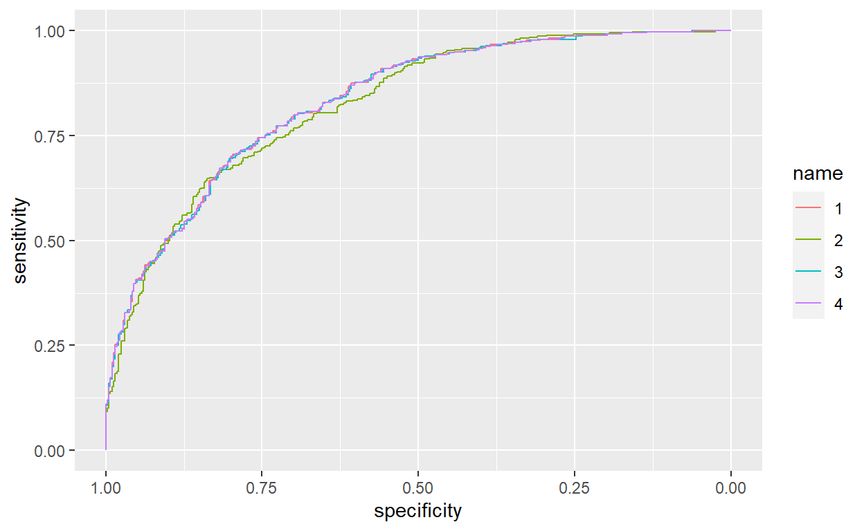
When interpreting a ROC curve, the goal is to approximate as closely as possible to the perfect classifier, which reaches 100% true positive at zero false positive. On the other hand, an estimator should perform better than the baseline, which is essentially a random guess.
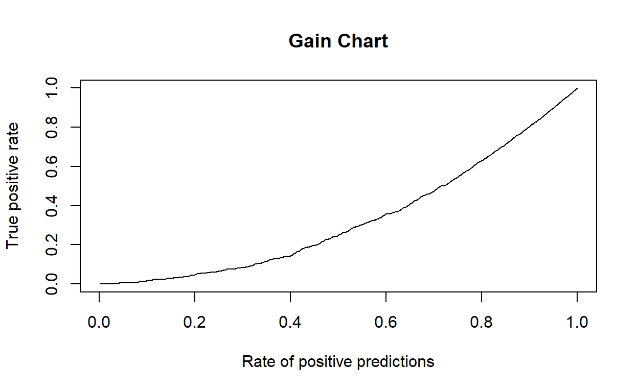
The Gain and Lift Charts
Gain
While the ROC curve provides a lot of detail into the performance of an estimator, and allows the performance of different estimators to be compared, we will sometimes want a different performance metric. For example, we may not have a sufficient budget to target all customers on which we have data. Thus, we can build a classifier to estimate which of our customers makes more than fifty thousand dollars a year. However, even this subset might be too large. What we really want is a way to select those instances from our classified data that we believe have the highest likelihood of being in our target category. Two charts that are useful to accomplish this goal are the gain chart and the related lift chart.
A classic example of where a lift chart is often used is in marketing. If we have a limited budget, we want to optimally target customers who will respond positively to ads or a marketing campaign. As a result, we would build a model and compute lift chart. This chart can be used to infer a cutoff point in the sample, above which we have the highest likelihood of a positive response. This will allow us to target customers optimally given a limited budget.
An alternative example is preventing customer churn, which is where customers migrate from one company to another. We can use a classifier to predict how likely a customer is to churn. With a lift chart, we can identify those customers most likely to churn and focus our limited retention budget on keeping them with our company.
pred<-ROCR::prediction(svmtestpred$high ,factor(svmtestpred$income2))

gain <- ROCR::performance(pred, "tpr", "rpp")

plot(gain, main = "Gain Chart")
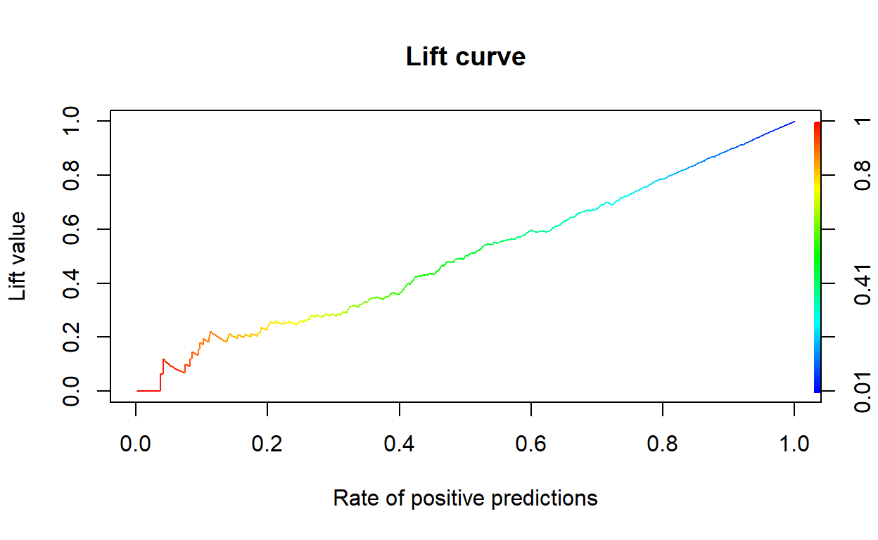
Lift
In the following Code chunk, we first compute the lift curve for our three different classification estimators. In this case, the lift is simply the gain for the estimator divided by the baseline response. To interpret the lift curve, recall that the value of the lift curve at any point indicates the relative improvement of our model over random.
From this curve, we can see that our default logistic regression and support vector classification algorithms both perform very well. But more importantly, if this classification was being used to target customers, we can optimize our results and use less money by targeting those customers who fall to the left in this chart. In some cases, you may see these curves converted into a profit curve, where the value of the prediction is included. In this example, we might assume a cost per targeted ad to convert the lift curve into a cost curve, which would allow us to determine how many (and who) of the individuals we should target given a budget. However, these types of curves are generally domain specific, so we do not present them in this notebook.
pred<-ROCR::prediction(svmtestpred$high ,factor(svmtestpred$income2))

perf <- ROCR::performance(pred,"lift","rpp")

plot(perf, main="Lift curve", colorize=T)
Don’t be afraid to search for better explanations.
Support Vector Machine: Regression
To this point, we have only applied the support vector machine algorithm to classification tasks. This algorithm can also be applied to regression tasks by using hyperplanes to model the data distribution. Basically, this algorithm works on regression problems by mapping the training data into a high dimensional space, which might involve a non-linear kernel, and performing something akin to linear regression on the data in this higher dimensional space. Recall that for best performance, SVMs require the data be normalized prior to use.
library(caret)
library(tidyverse)
#set the seed :)
set.seed(1)
#get our samples
#using the iris data
#lets split the data 60/40

trainIndex <- createDataPartition(iris$Sepal.Width, p = .6, list = FALSE, times = 1)

#look at the first few
#head(trainIndex)

#grab the data
SVMTrain <- iris[ trainIndex,]
SVMTest  <- iris[-trainIndex,]


iris_SVM <- train(
  form = Sepal.Width ~ Sepal.Length+Petal.Width+Petal.Length,
  data = SVMTrain,
  trControl = trainControl(method = "cv", number = 10),
  method = "svmRadial",
  preProcess = c("center", "scale"),
  tuneLength = 10)

iris_SVM
Support Vector Machines with Radial Basis Function Kernel

92 samples
 3 predictor

Pre-processing: centered (3), scaled (3)
Resampling: Cross-Validated (10 fold)
Summary of sample sizes: 82, 83, 83, 82, 82, 82, ...
Resampling results across tuning parameters:

  C       RMSE       Rsquared   MAE
    0.25  0.3045308  0.5760268  0.2312821
    0.50  0.2983330  0.5812156  0.2241842
    1.00  0.2958941  0.5832409  0.2237046
    2.00  0.2938179  0.5827772  0.2223655
    4.00  0.3009134  0.5676933  0.2288198
    8.00  0.3209230  0.5319581  0.2499194
   16.00  0.3372921  0.5113972  0.2638796
   32.00  0.3485226  0.4911218  0.2784212
   64.00  0.3810849  0.4388651  0.2993569
  128.00  0.4045562  0.3974911  0.3097310

Tuning parameter 'sigma' was held constant at a value of 1.966425
RMSE was used to select the optimal model using the smallest value.
The final values used for the model were sigma = 1.966425 and C = 2.summary(iris_SVM)
Length  Class   Mode
1 ksvm S4 svm_Pred<-predict(iris_SVM,SVMTest)
knitr::kable(svm_Pred)%>%
kableExtra::kable_styling("striped")%>%
kableExtra::scroll_box(width = "100%",height="300px")
| x |
|---|
| 3.322331 |
| 3.099127 |
| 3.391576 |
| 3.651888 |
| 3.049898 |
| 3.419540 |
| 3.365906 |
| 3.280495 |
| 3.038826 |
| 3.746301 |
| 3.620086 |
| 3.484209 |
| 3.446001 |
| 3.201112 |
| 3.691927 |
| 3.482859 |
| 3.506821 |
| 3.091146 |
| 3.599222 |
| 2.921077 |
| 3.074149 |
| 2.772444 |
| 2.640705 |
| 3.020858 |
| 2.535498 |
| 2.804590 |
| 3.012512 |
| 3.029405 |
| 2.631514 |
| 2.437158 |
| 2.709163 |
| 2.979379 |
| 2.723458 |
| 2.636843 |
| 2.722852 |
| 2.746948 |
| 2.799339 |
| 2.832003 |
| 2.445453 |
| 2.783559 |
| 3.068987 |
| 2.889967 |
| 3.078554 |
| 2.986732 |
| 2.865496 |
| 2.981215 |
| 2.954453 |
| 2.868738 |
| 2.983954 |
| 3.190911 |
| 3.084567 |
| 2.903104 |
| 3.010603 |
| 3.162211 |
| 3.182064 |
| 3.256616 |
| 2.924487 |
| 2.936688 |
svmtestpred<-cbind(svm_Pred,SVMTest)
#root mean squared error
RMSE(svmtestpred$svm_Pred,svmtestpred$Sepal.Width)
[1] 0.2791149#best measure ever...RSquared
cor(svmtestpred$svm_Pred,svmtestpred$Sepal.Width)^2
[1] 0.5812884👆😆
Exercise 3
- Run a regression using the adult data from the Classification: Adult Data section. Note: be sure to sample the data, i.e. use adult2.
fin