Regression

Introduction to Linear Regression

This lesson builds on the ordinary linear regression concept, introduced in business statistics, to discuss linear regression as a machine learning task. Regression, or the creation of a predictive model from data, is one of the key machine learning tasks. By using linear regression, which can often be solved analytically, we will introduce the concept of minimizing a cost function to determine the optimal model parameters in a straight-forward manner.

Objectives

By the end of this lesson, you will be able to

explain the role of the loss function in machine learning,
articulate how to compute a regression on multiple variables,
explain the different statistical measures that quantify the quality of a regression,
utilize categorical variables in a machine learning model, and
compute a linear regression model

You were introduced to the concept of linear regression by learning about simple linear regression. This initial approach treated linear regression as a statistical technique where the relation between independent variables (or features) and a dependent variable (or target) was determined by a mathematical relation. While powerful, the previous approach treated linear regression as a distinct, statistical approach to relating independent variables with a dependent variable. In this lesson, we instead treat linear regression as a machine learning task. As a result, we will use regression to fit a model to data. The model generated in this fashion can be explored in greater detail to either understand why the provided data follow the generated model (i.e., gain insight into the data), or the model can be used to generate new dependent values from future or unseen data (i.e., make predictions from the model).

We will use the tips data set. After loading this data, we display several rows, and next compute a simple linear regression to predict the tip feature from the total_bill feature.

For this section we need to load libraries:

library(tidyverse)
library(caret)

#load data. 
#curl package lets us download data from a website with the proper location
#check the packages tab and see if you have curl
#try following
  #?curl

library(curl)

load(curl("https://raw.githubusercontent.com/Professor-Hunt/ACC8143/main/data/tips.rda"))

head(tips,5)

# A tibble: 5 x 7
  total_bill   tip sex    smoker day   time    size
       <dbl> <dbl> <chr>  <chr>  <chr> <chr>  <dbl>
1       17.0  1.01 Female No     Sun   Dinner     2
2       10.3  1.66 Male   No     Sun   Dinner     3
3       21.0  3.5  Male   No     Sun   Dinner     3
4       23.7  3.31 Male   No     Sun   Dinner     2
5       24.6  3.61 Female No     Sun   Dinner     4

#view the whole dataset
knitr::kable(tips)%>%
  kableExtra::kable_styling("striped")%>%
  kableExtra::scroll_box(width = "100%",height="300px")

total_bill	tip	sex	smoker	day	time	size
16.99	1.01	Female	No	Sun	Dinner	2
10.34	1.66	Male	No	Sun	Dinner	3
21.01	3.50	Male	No	Sun	Dinner	3
23.68	3.31	Male	No	Sun	Dinner	2
24.59	3.61	Female	No	Sun	Dinner	4
25.29	4.71	Male	No	Sun	Dinner	4
8.77	2.00	Male	No	Sun	Dinner	2
26.88	3.12	Male	No	Sun	Dinner	4
15.04	1.96	Male	No	Sun	Dinner	2
14.78	3.23	Male	No	Sun	Dinner	2
10.27	1.71	Male	No	Sun	Dinner	2
35.26	5.00	Female	No	Sun	Dinner	4
15.42	1.57	Male	No	Sun	Dinner	2
18.43	3.00	Male	No	Sun	Dinner	4
14.83	3.02	Female	No	Sun	Dinner	2
21.58	3.92	Male	No	Sun	Dinner	2
10.33	1.67	Female	No	Sun	Dinner	3
16.29	3.71	Male	No	Sun	Dinner	3
16.97	3.50	Female	No	Sun	Dinner	3
20.65	3.35	Male	No	Sat	Dinner	3
17.92	4.08	Male	No	Sat	Dinner	2
20.29	2.75	Female	No	Sat	Dinner	2
15.77	2.23	Female	No	Sat	Dinner	2
39.42	7.58	Male	No	Sat	Dinner	4
19.82	3.18	Male	No	Sat	Dinner	2
17.81	2.34	Male	No	Sat	Dinner	4
13.37	2.00	Male	No	Sat	Dinner	2
12.69	2.00	Male	No	Sat	Dinner	2
21.70	4.30	Male	No	Sat	Dinner	2
19.65	3.00	Female	No	Sat	Dinner	2
9.55	1.45	Male	No	Sat	Dinner	2
18.35	2.50	Male	No	Sat	Dinner	4
15.06	3.00	Female	No	Sat	Dinner	2
20.69	2.45	Female	No	Sat	Dinner	4
17.78	3.27	Male	No	Sat	Dinner	2
24.06	3.60	Male	No	Sat	Dinner	3
16.31	2.00	Male	No	Sat	Dinner	3
16.93	3.07	Female	No	Sat	Dinner	3
18.69	2.31	Male	No	Sat	Dinner	3
31.27	5.00	Male	No	Sat	Dinner	3
16.04	2.24	Male	No	Sat	Dinner	3
17.46	2.54	Male	No	Sun	Dinner	2
13.94	3.06	Male	No	Sun	Dinner	2
9.68	1.32	Male	No	Sun	Dinner	2
30.40	5.60	Male	No	Sun	Dinner	4
18.29	3.00	Male	No	Sun	Dinner	2
22.23	5.00	Male	No	Sun	Dinner	2
32.40	6.00	Male	No	Sun	Dinner	4
28.55	2.05	Male	No	Sun	Dinner	3
18.04	3.00	Male	No	Sun	Dinner	2
12.54	2.50	Male	No	Sun	Dinner	2
10.29	2.60	Female	No	Sun	Dinner	2
34.81	5.20	Female	No	Sun	Dinner	4
9.94	1.56	Male	No	Sun	Dinner	2
25.56	4.34	Male	No	Sun	Dinner	4
19.49	3.51	Male	No	Sun	Dinner	2
38.01	3.00	Male	Yes	Sat	Dinner	4
26.41	1.50	Female	No	Sat	Dinner	2
11.24	1.76	Male	Yes	Sat	Dinner	2
48.27	6.73	Male	No	Sat	Dinner	4
20.29	3.21	Male	Yes	Sat	Dinner	2
13.81	2.00	Male	Yes	Sat	Dinner	2
11.02	1.98	Male	Yes	Sat	Dinner	2
18.29	3.76	Male	Yes	Sat	Dinner	4
17.59	2.64	Male	No	Sat	Dinner	3
20.08	3.15	Male	No	Sat	Dinner	3
16.45	2.47	Female	No	Sat	Dinner	2
3.07	1.00	Female	Yes	Sat	Dinner	1
20.23	2.01	Male	No	Sat	Dinner	2
15.01	2.09	Male	Yes	Sat	Dinner	2
12.02	1.97	Male	No	Sat	Dinner	2
17.07	3.00	Female	No	Sat	Dinner	3
26.86	3.14	Female	Yes	Sat	Dinner	2
25.28	5.00	Female	Yes	Sat	Dinner	2
14.73	2.20	Female	No	Sat	Dinner	2
10.51	1.25	Male	No	Sat	Dinner	2
17.92	3.08	Male	Yes	Sat	Dinner	2
27.20	4.00	Male	No	Thur	Lunch	4
22.76	3.00	Male	No	Thur	Lunch	2
17.29	2.71	Male	No	Thur	Lunch	2
19.44	3.00	Male	Yes	Thur	Lunch	2
16.66	3.40	Male	No	Thur	Lunch	2
10.07	1.83	Female	No	Thur	Lunch	1
32.68	5.00	Male	Yes	Thur	Lunch	2
15.98	2.03	Male	No	Thur	Lunch	2
34.83	5.17	Female	No	Thur	Lunch	4
13.03	2.00	Male	No	Thur	Lunch	2
18.28	4.00	Male	No	Thur	Lunch	2
24.71	5.85	Male	No	Thur	Lunch	2
21.16	3.00	Male	No	Thur	Lunch	2
28.97	3.00	Male	Yes	Fri	Dinner	2
22.49	3.50	Male	No	Fri	Dinner	2
5.75	1.00	Female	Yes	Fri	Dinner	2
16.32	4.30	Female	Yes	Fri	Dinner	2
22.75	3.25	Female	No	Fri	Dinner	2
40.17	4.73	Male	Yes	Fri	Dinner	4
27.28	4.00	Male	Yes	Fri	Dinner	2
12.03	1.50	Male	Yes	Fri	Dinner	2
21.01	3.00	Male	Yes	Fri	Dinner	2
12.46	1.50	Male	No	Fri	Dinner	2
11.35	2.50	Female	Yes	Fri	Dinner	2
15.38	3.00	Female	Yes	Fri	Dinner	2
44.30	2.50	Female	Yes	Sat	Dinner	3
22.42	3.48	Female	Yes	Sat	Dinner	2
20.92	4.08	Female	No	Sat	Dinner	2
15.36	1.64	Male	Yes	Sat	Dinner	2
20.49	4.06	Male	Yes	Sat	Dinner	2
25.21	4.29	Male	Yes	Sat	Dinner	2
18.24	3.76	Male	No	Sat	Dinner	2
14.31	4.00	Female	Yes	Sat	Dinner	2
14.00	3.00	Male	No	Sat	Dinner	2
7.25	1.00	Female	No	Sat	Dinner	1
38.07	4.00	Male	No	Sun	Dinner	3
23.95	2.55	Male	No	Sun	Dinner	2
25.71	4.00	Female	No	Sun	Dinner	3
17.31	3.50	Female	No	Sun	Dinner	2
29.93	5.07	Male	No	Sun	Dinner	4
10.65	1.50	Female	No	Thur	Lunch	2
12.43	1.80	Female	No	Thur	Lunch	2
24.08	2.92	Female	No	Thur	Lunch	4
11.69	2.31	Male	No	Thur	Lunch	2
13.42	1.68	Female	No	Thur	Lunch	2
14.26	2.50	Male	No	Thur	Lunch	2
15.95	2.00	Male	No	Thur	Lunch	2
12.48	2.52	Female	No	Thur	Lunch	2
29.80	4.20	Female	No	Thur	Lunch	6
8.52	1.48	Male	No	Thur	Lunch	2
14.52	2.00	Female	No	Thur	Lunch	2
11.38	2.00	Female	No	Thur	Lunch	2
22.82	2.18	Male	No	Thur	Lunch	3
19.08	1.50	Male	No	Thur	Lunch	2
20.27	2.83	Female	No	Thur	Lunch	2
11.17	1.50	Female	No	Thur	Lunch	2
12.26	2.00	Female	No	Thur	Lunch	2
18.26	3.25	Female	No	Thur	Lunch	2
8.51	1.25	Female	No	Thur	Lunch	2
10.33	2.00	Female	No	Thur	Lunch	2
14.15	2.00	Female	No	Thur	Lunch	2
16.00	2.00	Male	Yes	Thur	Lunch	2
13.16	2.75	Female	No	Thur	Lunch	2
17.47	3.50	Female	No	Thur	Lunch	2
34.30	6.70	Male	No	Thur	Lunch	6
41.19	5.00	Male	No	Thur	Lunch	5
27.05	5.00	Female	No	Thur	Lunch	6
16.43	2.30	Female	No	Thur	Lunch	2
8.35	1.50	Female	No	Thur	Lunch	2
18.64	1.36	Female	No	Thur	Lunch	3
11.87	1.63	Female	No	Thur	Lunch	2
9.78	1.73	Male	No	Thur	Lunch	2
7.51	2.00	Male	No	Thur	Lunch	2
14.07	2.50	Male	No	Sun	Dinner	2
13.13	2.00	Male	No	Sun	Dinner	2
17.26	2.74	Male	No	Sun	Dinner	3
24.55	2.00	Male	No	Sun	Dinner	4
19.77	2.00	Male	No	Sun	Dinner	4
29.85	5.14	Female	No	Sun	Dinner	5
48.17	5.00	Male	No	Sun	Dinner	6
25.00	3.75	Female	No	Sun	Dinner	4
13.39	2.61	Female	No	Sun	Dinner	2
16.49	2.00	Male	No	Sun	Dinner	4
21.50	3.50	Male	No	Sun	Dinner	4
12.66	2.50	Male	No	Sun	Dinner	2
16.21	2.00	Female	No	Sun	Dinner	3
13.81	2.00	Male	No	Sun	Dinner	2
17.51	3.00	Female	Yes	Sun	Dinner	2
24.52	3.48	Male	No	Sun	Dinner	3
20.76	2.24	Male	No	Sun	Dinner	2
31.71	4.50	Male	No	Sun	Dinner	4
10.59	1.61	Female	Yes	Sat	Dinner	2
10.63	2.00	Female	Yes	Sat	Dinner	2
50.81	10.00	Male	Yes	Sat	Dinner	3
15.81	3.16	Male	Yes	Sat	Dinner	2
7.25	5.15	Male	Yes	Sun	Dinner	2
31.85	3.18	Male	Yes	Sun	Dinner	2
16.82	4.00	Male	Yes	Sun	Dinner	2
32.90	3.11	Male	Yes	Sun	Dinner	2
17.89	2.00	Male	Yes	Sun	Dinner	2
14.48	2.00	Male	Yes	Sun	Dinner	2
9.60	4.00	Female	Yes	Sun	Dinner	2
34.63	3.55	Male	Yes	Sun	Dinner	2
34.65	3.68	Male	Yes	Sun	Dinner	4
23.33	5.65	Male	Yes	Sun	Dinner	2
45.35	3.50	Male	Yes	Sun	Dinner	3
23.17	6.50	Male	Yes	Sun	Dinner	4
40.55	3.00	Male	Yes	Sun	Dinner	2
20.69	5.00	Male	No	Sun	Dinner	5
20.90	3.50	Female	Yes	Sun	Dinner	3
30.46	2.00	Male	Yes	Sun	Dinner	5
18.15	3.50	Female	Yes	Sun	Dinner	3
23.10	4.00	Male	Yes	Sun	Dinner	3
15.69	1.50	Male	Yes	Sun	Dinner	2
19.81	4.19	Female	Yes	Thur	Lunch	2
28.44	2.56	Male	Yes	Thur	Lunch	2
15.48	2.02	Male	Yes	Thur	Lunch	2
16.58	4.00	Male	Yes	Thur	Lunch	2
7.56	1.44	Male	No	Thur	Lunch	2
10.34	2.00	Male	Yes	Thur	Lunch	2
43.11	5.00	Female	Yes	Thur	Lunch	4
13.00	2.00	Female	Yes	Thur	Lunch	2
13.51	2.00	Male	Yes	Thur	Lunch	2
18.71	4.00	Male	Yes	Thur	Lunch	3
12.74	2.01	Female	Yes	Thur	Lunch	2
13.00	2.00	Female	Yes	Thur	Lunch	2
16.40	2.50	Female	Yes	Thur	Lunch	2
20.53	4.00	Male	Yes	Thur	Lunch	4
16.47	3.23	Female	Yes	Thur	Lunch	3
26.59	3.41	Male	Yes	Sat	Dinner	3
38.73	3.00	Male	Yes	Sat	Dinner	4
24.27	2.03	Male	Yes	Sat	Dinner	2
12.76	2.23	Female	Yes	Sat	Dinner	2
30.06	2.00	Male	Yes	Sat	Dinner	3
25.89	5.16	Male	Yes	Sat	Dinner	4
48.33	9.00	Male	No	Sat	Dinner	4
13.27	2.50	Female	Yes	Sat	Dinner	2
28.17	6.50	Female	Yes	Sat	Dinner	3
12.90	1.10	Female	Yes	Sat	Dinner	2
28.15	3.00	Male	Yes	Sat	Dinner	5
11.59	1.50	Male	Yes	Sat	Dinner	2
7.74	1.44	Male	Yes	Sat	Dinner	2
30.14	3.09	Female	Yes	Sat	Dinner	4
12.16	2.20	Male	Yes	Fri	Lunch	2
13.42	3.48	Female	Yes	Fri	Lunch	2
8.58	1.92	Male	Yes	Fri	Lunch	1
15.98	3.00	Female	No	Fri	Lunch	3
13.42	1.58	Male	Yes	Fri	Lunch	2
16.27	2.50	Female	Yes	Fri	Lunch	2
10.09	2.00	Female	Yes	Fri	Lunch	2
20.45	3.00	Male	No	Sat	Dinner	4
13.28	2.72	Male	No	Sat	Dinner	2
22.12	2.88	Female	Yes	Sat	Dinner	2
24.01	2.00	Male	Yes	Sat	Dinner	4
15.69	3.00	Male	Yes	Sat	Dinner	3
11.61	3.39	Male	No	Sat	Dinner	2
10.77	1.47	Male	No	Sat	Dinner	2
15.53	3.00	Male	Yes	Sat	Dinner	2
10.07	1.25	Male	No	Sat	Dinner	2
12.60	1.00	Male	Yes	Sat	Dinner	2
32.83	1.17	Male	Yes	Sat	Dinner	2
35.83	4.67	Female	No	Sat	Dinner	3
29.03	5.92	Male	No	Sat	Dinner	3
27.18	2.00	Female	Yes	Sat	Dinner	2
22.67	2.00	Male	Yes	Sat	Dinner	2
17.82	1.75	Male	No	Sat	Dinner	2
18.78	3.00	Female	No	Thur	Dinner	2

Perform simple linear regression

OLS1<-lm(formula=tip~total_bill,data=tips)
#general output
OLS1


Call:
lm(formula = tip ~ total_bill, data = tips)

Coefficients:
(Intercept)   total_bill  
     0.9203       0.1050

#more common output
summary(OLS1)


Call:
lm(formula = tip ~ total_bill, data = tips)

Residuals:
    Min      1Q  Median      3Q     Max 
-3.1982 -0.5652 -0.0974  0.4863  3.7434 

Coefficients:
            Estimate Std. Error t value Pr(>|t|)    
(Intercept) 0.920270   0.159735   5.761 2.53e-08 ***
total_bill  0.105025   0.007365  14.260  < 2e-16 ***
---
Signif. codes:  0 '***' 0.001 '**' 0.01 '*' 0.05 '.' 0.1 ' ' 1

Residual standard error: 1.022 on 242 degrees of freedom
Multiple R-squared:  0.4566,    Adjusted R-squared:  0.4544 
F-statistic: 203.4 on 1 and 242 DF,  p-value: < 2.2e-16

#correlation or R-squared...
cor(tips$total_bill,tips$tip)^2

[1] 0.4566166

Formalism

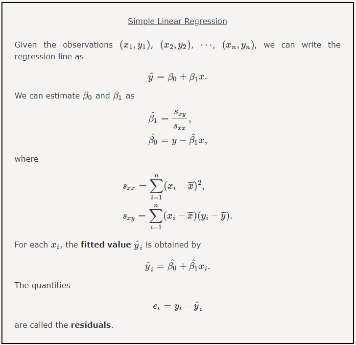
Formally, this simple linear model related the independent variables \(x_i\) to the dependent variables \(y_i\) in our data set via two parameters: an intercept, and a slope. Mathematically, we express this relation in the following form:

\[ f(x_i) = \beta * x_i + \alpha + \epsilon_i \]

where \(\epsilon_i\) accounts for the difference between the model and the data for each data point \((x_i,y_i)\). If we have a perfect model, these errors, \(\epsilon_i\), are all zero, and \(y_i = f(x_i)\). In real life, however, the error terms rarely vanish because even if the original relationship is perfect noise creeps into the measurement process.

As a result, in this simple example we wish to determine the model parameters: \(\beta_i\), and \(\alpha_i\) that minimize the values of \(\epsilon_i\). We could perform this process in an iterative manner, trying different values for the model parameters and measuring the error function. This approach is often used in machine learning, where we define a cost function that we seek to minimize by selecting the best model parameters.

In the case of a simple linear model, we have several potential cost (or loss) functions that we could seek to minimize, but we will use the common l2-norm: \(\epsilon_i^2 = \left( \ y_i - f(x_i) \ \right)^2\), where \(f(x_i)\) is defined by our model parameters. We demonstrate this approach visually in the following code block, where we minimize the sum of the l2-norm model residuals, which is done by finding the best model parameters: \(\hat{\beta}\), and \(\hat{\alpha}\).

Formulas 😢

#Get some data
AnsDat<-anscombe%>%
  select(y1,x1)

#extract x and y columns
Y<-AnsDat$y1
X<-AnsDat$x1

#find the number of data points
n<-nrow(AnsDat)

#determine mean values
mean_x<-mean(X,na.rm = TRUE)
mean_y<-mean(Y,na.rm = TRUE)

#determine best fit model parameters (from simple linear regression)
beta = sum((X - mean_x) * (Y - mean_y)) / sum((X - mean_x)**2)
beta

[1] 0.5000909

alpha = mean_y - beta * mean_x
alpha

[1] 3.000091

#lets double check
summary(lm(formula=Y~X,data=AnsDat))


Call:
lm(formula = Y ~ X, data = AnsDat)

Residuals:
     Min       1Q   Median       3Q      Max 
-1.92127 -0.45577 -0.04136  0.70941  1.83882 

Coefficients:
            Estimate Std. Error t value Pr(>|t|)   
(Intercept)   3.0001     1.1247   2.667  0.02573 * 
X             0.5001     0.1179   4.241  0.00217 **
---
Signif. codes:  0 '***' 0.001 '**' 0.01 '*' 0.05 '.' 0.1 ' ' 1

Residual standard error: 1.237 on 9 degrees of freedom
Multiple R-squared:  0.6665,    Adjusted R-squared:  0.6295 
F-statistic: 17.99 on 1 and 9 DF,  p-value: 0.00217

Plots

library(ggplot2)

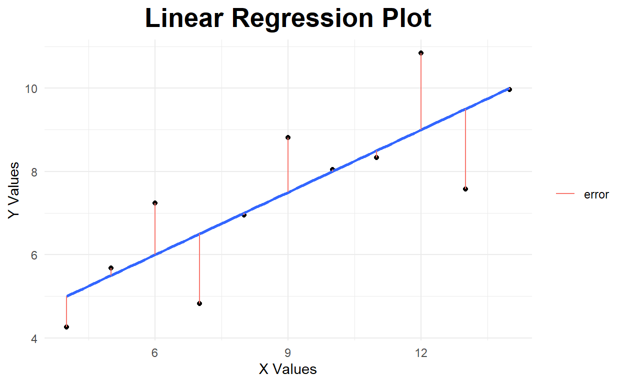
#create regression plot
ggplot(AnsDat,aes(x1, y1)) +
  geom_point() +
  geom_smooth(method='lm', se=FALSE) +
  geom_segment(aes(x=X, xend=X, y=Y, yend=lm(Y~X)$fitted.values, color="error"))+
  theme_minimal() +
  labs(x='X Values', y='Y Values', title='Linear Regression Plot') +
  theme(plot.title = element_text(hjust=0.5, size=20, face='bold')) + 
  theme(legend.title = element_blank())

Cost Function

This simple example demonstrates a fundamental concept in machine learning, namely the minimization of a cost (or loss) function, which quantifies how well a model represents a data set. For a given data set, the cost function is completely specified by the model parameters, thus a more complex model has a more complex cost function, which can become difficult to minimize. To clarify this point, we now turn to the exploration of the shape of cost functions.

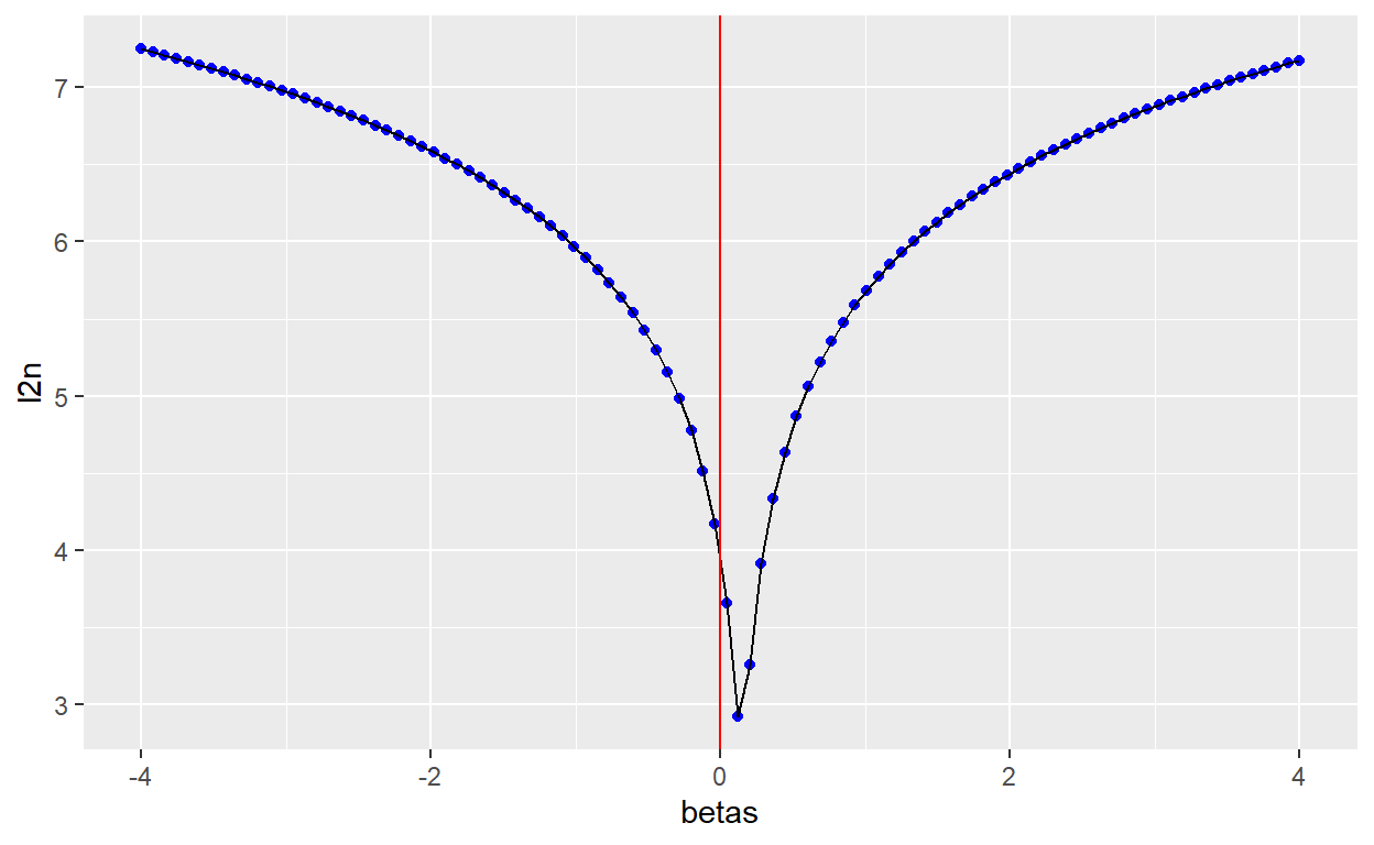
For simplicity, we start with a one-dimensional cost function, a linear model with no intercept: \(f(x_i) = \beta x_i\). In the following code cell, we compute the cost function for a given data set as a function of the unknown parameter \(\beta\). In this case, the minimum is easy to visualize, given the steepness of the cost function around the minimum.

#define our betas
betas<-seq(-4,4,length.out=100)

#define our cost function
l2n = sapply(as.matrix(betas), function(m) log(sqrt(sum((as.matrix(tips$tip) - m*as.matrix(tips$total_bill))^2))))  # The L2-norm

library(ggplot2)
costplot<-as.data.frame(cbind(betas,l2n))
#create regression plot
ggplot(costplot,aes(betas, l2n)) +
  geom_point(color="blue") + geom_line()+
  geom_vline(xintercept=0, color="red")

In general, however, we face two challenges:

the cost function will likely be more complex, and
our data will be higher dimensional.

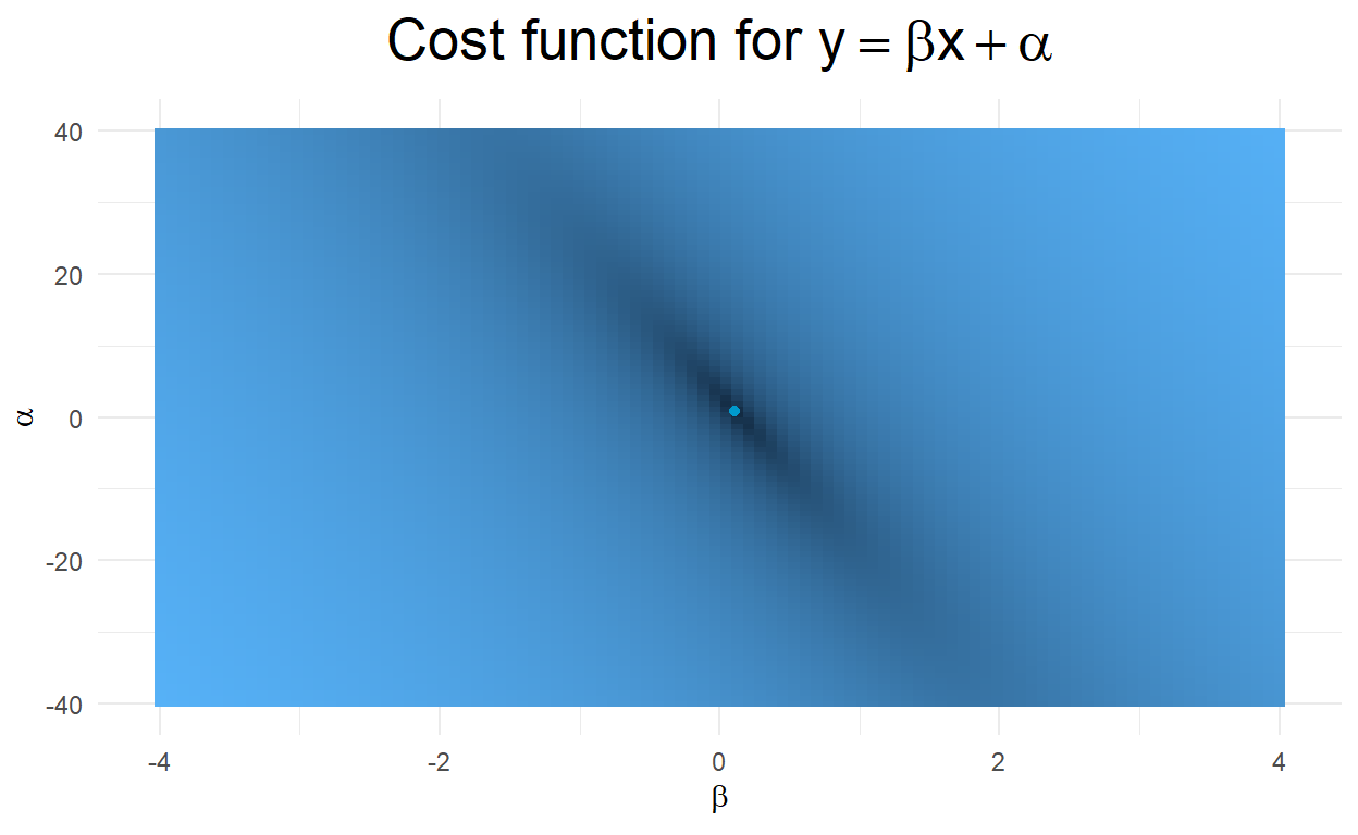
In general, we must employ a (potentially) complex mathematical technique to find the (hopefully) global minimum of the cost function. We can increase the complexity of our cost function analysis by extending the original model to include both a slope and an intercept. We now must find the minimum of this two dimensional model, given our observed data. We do this in the following code cell where we generate a grid of values in our two parameters, and compute the cost function for these different parameter combinations.

To display the data which generates a sampling grid across potential values for the slope \(\beta\) and intercept \(\alpha\) in our model. We once again vectorize our cost function and broadcast it across the sampling grid. We accumulate the cost at each grid point and generate a two-dimensional image of the values of the cost function across our sampling grid. To make the image appear cleaner, we perform Gaussian interpolation between sample points.

As the following two-dimensional image displays, our cost function is not aligned with either parameter, but is steeper in the slope parameter and less steep in the intercept parameter. Thus, we would expect that small changes in the slope will quickly increase our cost (which we saw in the previous one-dimensional example), while small changes in the intercept will produce smaller changes in our cost function (note that the range for intercepts is much larger than the range for the slope parameters).

#define our betas
betas<-seq(-4,4,length.out=100)
alphas<-seq(-40,40,length.out=100)
## Generate a grid of X- and Y- values on which to predict
grid <-expand.grid(betas,alphas)
#define our cost function
l2n2 = mapply( function(m,b) log(sqrt(sum((as.matrix(tips$tip) - m*as.matrix(tips$total_bill) - b)^2))),as.matrix(grid$Var1),as.matrix(grid$Var2))  # The L2-norm

library(ggplot2)

ggplot(grid, aes(Var1, Var2)) +
  geom_raster(aes(fill=l2n2),show.legend = FALSE) +
  geom_point(color="deepskyblue3",aes(OLS1$coefficients[[2]],OLS1$coefficients[[1]]))+
  theme_minimal() +
  labs(x=expression(beta), y=expression(alpha), title=expression(paste("Cost function for"," ",y==beta*x+alpha))) +
  theme(plot.title = element_text(hjust=0.5, size=20, face='bold')) + 
  theme(legend.title = element_blank())

As we move to higher dimensional data sets or more complex cost functions, the challenge of finding the global minimum becomes increasingly difficult. As a result, many mathematical techniques have been developed to find the global minimum of a (potentially) complex function. The standard approach is gradient descent, where we use the fact that the first derivative (or gradient) measures the slope of a function at a given point. We can use the slope to infer which direction is downhill and thus travel (hopefully) towards the minimum.

A major challenge with this approach is the potential to become stuck in a local and not global minima. Thus, modifications are often added to reduce the likelihood of becoming stuck in a local minimum. One popular example of this approach is known as stochastic gradient descent. This algorithm employs standard gradient descent, but adds an occasional random jump in the parameter space to reduce the chances of being stuck in a local valley. Another, very different, approach to this problem is the use of genetic algorithms, which employ techniques from evolutionary biology to minimize the cost function.

For a mental picture of this process, imagine hiking in the mountains and flip the challenge to finding the highest peak, so we will use gradient ascent. Gradient ascent is similar to finding the local mountain peak and climbing it. This local peak might look like it is the largest, but a random jump away from the local peak might enable one to view much larger peaks beyond, which can subsequently be climbed with a new gradient ascent.

Whenever you perform machine learning in the future, you should keep in mind that the model that you generate for a given data set has generally resulted from the minimization of a cost function. Thus, there remains the possibility that with more effort, more data, or a better cost minimization strategy, a new, and better model may potentially exist.

#set the seed :)
set.seed(1)
#get our samples

#lets split the data 60/40
library(caret)
trainIndex <- createDataPartition(tips$tip, p = .6, list = FALSE, times = 1)

#look at the first few
#head(trainIndex)

#grab the data
tipsTrain <- tips[ trainIndex,]
tipsTest  <- tips[-trainIndex,]

Linear Regression

In the following code cells, we use the lm estimator to fit our sample data, plot the results, and finally display the fit coefficients.

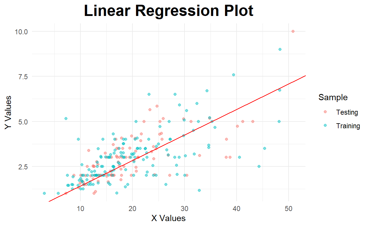
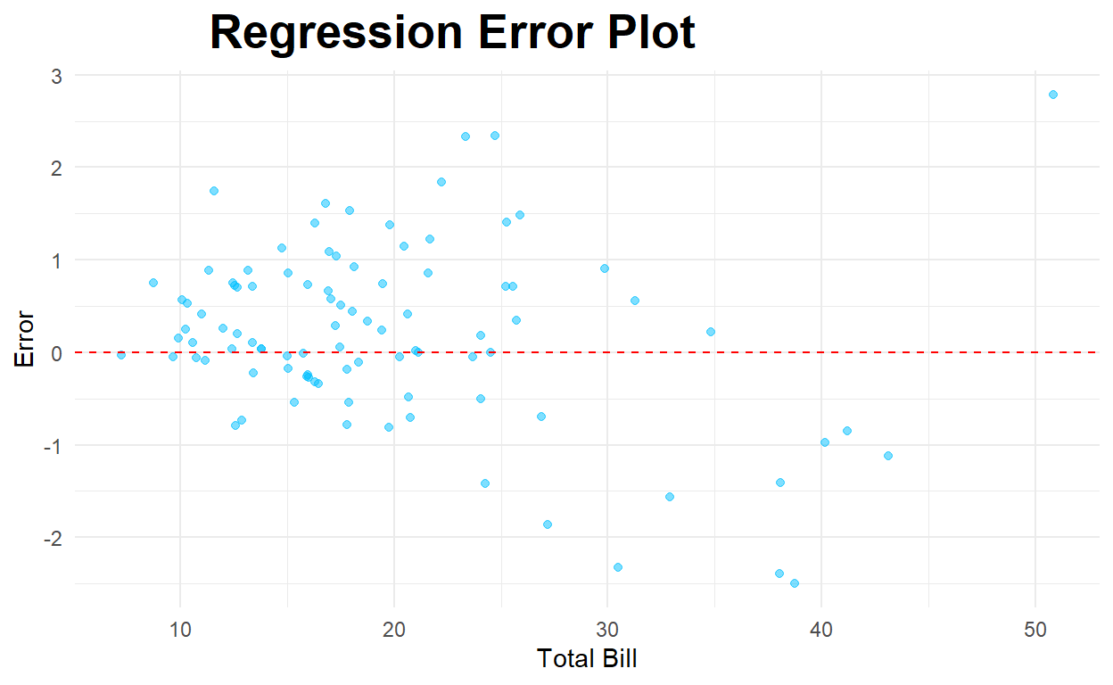
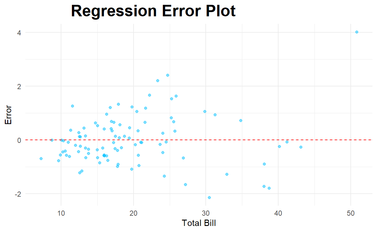
The first code cell defines a function that will make two plots. The top plot is a comparison between a single independent variable (Total Bill) and the dependent variable (Tip). This plot differentiates the training data, the testing data, and the linear model. The bottom plot displays the model residuals (dependent variable - model result) as a function of the independent variable. The primary benefit of this plot is the ability to identify any structure in the residuals, which can indicate a bad model. For example, if the residual plot shows a linear relationship, that indicates the original model incorrectly related the independent and dependent variables.

In the following code cells, we first compute a linear fit with no intercept, after which we compute a linear fit with both a slope and an intercept. The fit results are displayed as well as the regression and residual plots.

The code below computes a regression with no intercept.

#fit simple linear regression model
model_noint <- lm(tip ~ 0+total_bill , data = tipsTrain)

noint_results<-predict(model_noint,tipsTest)
###compute fit
summary(model_noint)


Call:
lm(formula = tip ~ 0 + total_bill, data = tipsTrain)

Residuals:
    Min      1Q  Median      3Q     Max 
-3.7910 -0.1871  0.2019  0.7518  4.1204 

Coefficients:
           Estimate Std. Error t value Pr(>|t|)    
total_bill 0.142010   0.004331   32.79   <2e-16 ***
---
Signif. codes:  0 '***' 0.001 '**' 0.01 '*' 0.05 '.' 0.1 ' ' 1

Residual standard error: 1.153 on 147 degrees of freedom
Multiple R-squared:  0.8797,    Adjusted R-squared:  0.8789 
F-statistic:  1075 on 1 and 147 DF,  p-value: < 2.2e-16

knitr::kable(caret::RMSE(noint_results,tipsTest$tip),col.names = "RMSE")

RMSE
0.9808281

Below is the regression plot for the model with no intercept.

tipsTest$Sample<-"Testing"
tipsTrain$Sample<-"Training"

Combined_Tips<-rbind(tipsTest,tipsTrain)
#create regression plot with customized style
ggplot(Combined_Tips,aes(x=total_bill, y=tip,color=Sample)) +
  geom_point(alpha=.5) +
  theme_minimal() +
  labs(x='X Values', y='Y Values', title='Linear Regression Plot') +
  theme(plot.title = element_text(hjust=0.5, size=20, face='bold')) +
  geom_abline(aes(slope=model_noint$coefficients[[1]],intercept=0),color="red")

Below is a residual (error) plot.

library(tidyverse)
#create residuals
testwithpred<-as.data.frame(cbind(noint_results,tipsTest))
#create residuals
testwithpred<-testwithpred%>%
  rename(prediction=noint_results)%>%
  mutate(error=tip-prediction)

#create regression plot with customized style
ggplot(testwithpred,aes(x=total_bill, y=error)) +
  geom_point(alpha=.5,color="deepskyblue") +
  theme_minimal() +
  labs(x='Total Bill', y='Error', title='Regression Error Plot') +
  theme(plot.title = element_text(hjust=0.25, size=20, face='bold')) +
  geom_hline(yintercept=0,color="red",linetype="dashed")

Link to some good examples of interpreting residual plots 🏫

Model with an intercept

#fit simple linear regression model
model_int <- lm(tip ~ total_bill , data = tipsTrain)

int_results<-predict(model_int,tipsTest)
###compute fit
summary(model_int)


Call:
lm(formula = tip ~ total_bill, data = tipsTrain)

Residuals:
    Min      1Q  Median      3Q     Max 
-3.1243 -0.5729 -0.0703  0.4668  3.4083 

Coefficients:
            Estimate Std. Error t value Pr(>|t|)    
(Intercept) 1.018249   0.209997   4.849 3.14e-06 ***
total_bill  0.099788   0.009596  10.399  < 2e-16 ***
---
Signif. codes:  0 '***' 0.001 '**' 0.01 '*' 0.05 '.' 0.1 ' ' 1

Residual standard error: 1.074 on 146 degrees of freedom
Multiple R-squared:  0.4255,    Adjusted R-squared:  0.4216 
F-statistic: 108.1 on 1 and 146 DF,  p-value: < 2.2e-16

knitr::kable(caret::RMSE(int_results,tipsTest$tip),col.names = "RMSE")

RMSE
0.9408934

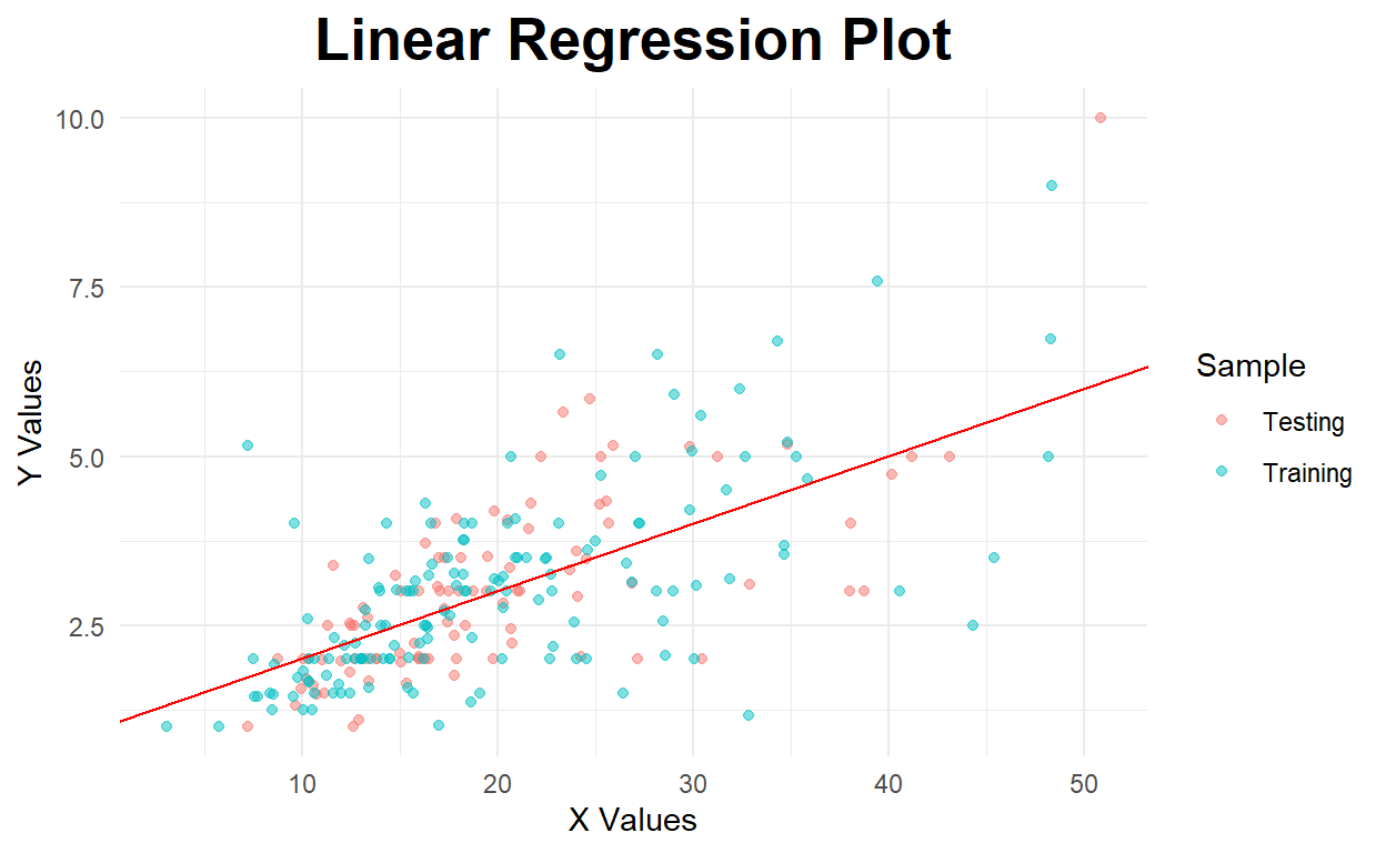
Below is a model with an intercept

#create regression plot with customized style
ggplot(Combined_Tips,aes(x=total_bill, y=tip,color=Sample)) +
  geom_point(alpha=.5) +
  theme_minimal() +
  labs(x='X Values', y='Y Values', title='Linear Regression Plot') +
  theme(plot.title = element_text(hjust=0.5, size=20, face='bold')) +
  geom_abline(aes(slope=model_int$coefficients[[2]],intercept=model_int$coefficients[[1]]),color="red")

Residual Plot

#create residuals
testwithpred2<-as.data.frame(cbind(int_results,tipsTest))
#create residuals
testwithpred2<-testwithpred2%>%
  rename(prediction=int_results)%>%
  mutate(error=tip-prediction)

#create regression plot with customized style
ggplot(testwithpred2,aes(x=total_bill, y=error)) +
  geom_point(alpha=.5,color="deepskyblue") +
  theme_minimal() +
  labs(x='Total Bill', y='Error', title='Regression Error Plot') +
  theme(plot.title = element_text(hjust=0.25, size=20, face='bold')) +
  geom_hline(yintercept=0,color="red",linetype="dashed")

Multivariate Regression

Often, using more data will result in more accurate models, since finer details can be captured. For example, if we see structure in a residual plot, the easiest solution is often to add additional independent variables to our model, which results in a multivariate linear regression model. The only major change required to our previous model building code is the expansion of our equation in the lm() function to include the additional independent variables.

To demonstrate building a multi-variate regression model, the following code uses both the total_bill and size features from the tips data set to use as independent variables. The tip feature is used as the dependent variable.

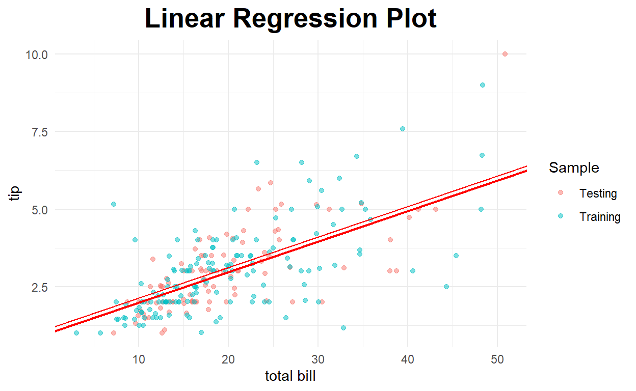
The following code generates a multi-variate linear model, displays the model parameters, and displays the regression and residual plots. To make the regression plot, we must use only one feature (in this case the total_bill). As a result, when we display the generated model, we get a series of lines that are the projections of the multi-variate model on this two-dimensional figure.

#fit simple linear regression model
model_multi <- lm(tip ~ total_bill+size , data = tipsTrain)

multi_results<-predict(model_multi,tipsTest)
###compute fit
summary(model_multi)


Call:
lm(formula = tip ~ total_bill + size, data = tipsTrain)

Residuals:
    Min      1Q  Median      3Q     Max 
-2.5272 -0.5926 -0.0678  0.5428  3.3375 

Coefficients:
            Estimate Std. Error t value Pr(>|t|)    
(Intercept)  0.46842    0.24272   1.930 0.055576 .  
total_bill   0.07291    0.01135   6.425 1.77e-09 ***
size         0.41764    0.10448   3.997 0.000102 ***
---
Signif. codes:  0 '***' 0.001 '**' 0.01 '*' 0.05 '.' 0.1 ' ' 1

Residual standard error: 1.023 on 145 degrees of freedom
Multiple R-squared:  0.4825,    Adjusted R-squared:  0.4754 
F-statistic:  67.6 on 2 and 145 DF,  p-value: < 2.2e-16

knitr::kable(caret::RMSE(multi_results,tipsTest$tip),col.names = "RMSE")

RMSE
1.039275

library(plotly)

scatter.plot<-plot_ly(Combined_Tips, x = ~total_bill, y = ~size, z = ~tip, color = ~Sample, colors = c('lightblue', 'violet'))%>% 
  add_markers(size=6)%>% 
  layout(scene = list(
          xaxis = list(title = 'Total Bill'),
          yaxis = list(title = 'Size'),
          zaxis = list(title = 'Tip')))

#scatter.plot

library(reshape2)
#Graph Resolution (more important for more complex shapes)
graph_reso <- 0.05

#Setup Axis
axis_x <- seq(min(tipsTest$total_bill), max(tipsTest$total_bill), by = graph_reso)
axis_y <- seq(min(tipsTest$size), max(tipsTest$size), by = graph_reso)

#Sample points
lm_surface <- expand.grid(total_bill = axis_x,size = axis_y,KEEP.OUT.ATTRS = F)
lm_surface$tips <- predict(model_multi, newdata = lm_surface)
lm_surface <- acast(lm_surface, size ~ total_bill, value.var = "tips")

scatter.plot<- add_trace(p = scatter.plot,
                       z = lm_surface,
                       x = axis_x,
                       y = axis_y,
                       type = "surface",colorscale = list(c(0, 1), c("wheat", "royalblue")))%>%
                layout(legend = list(x = -.1, y = 1), title="Regression Plot")

scatter.plot

#create residuals
testwithpred3<-as.data.frame(cbind(multi_results,tipsTest))
#create residuals
testwithpred3<-testwithpred3%>%
  rename(prediction=multi_results)%>%
  mutate(error=tip-prediction)


library(plotly)

scatter.plot<-plot_ly(testwithpred3, x = ~total_bill, y = ~size, z = ~error)%>% 
  add_markers(size=6)%>% 
  layout(scene = list(
          xaxis = list(title = 'Total Bill'),
          yaxis = list(title = 'Size'),
          zaxis = list(title = 'Error')))

#scatter.plot

library(reshape2)
#Graph Resolution (more important for more complex shapes)
graph_reso <- 0.05

#Setup Axis
axis_x <- seq(min(tipsTest$total_bill), max(tipsTest$total_bill), by = graph_reso)
axis_y <- seq(min(tipsTest$size), max(tipsTest$size), by = graph_reso)

#Sample points
lm_surface <- expand.grid(total_bill = axis_x,size = axis_y,KEEP.OUT.ATTRS = F)
lm_surface$error <-rep(0,nrow(lm_surface))
lm_surface <- acast(lm_surface, size ~ total_bill, value.var = "error")

scatter.plot<- add_trace(p = scatter.plot,
                       z = lm_surface,
                       x = axis_x,
                       y = axis_y,
                       type = "surface",
                       colorscale = list(c(0,1), c("red","red")))%>%
                       layout(showlegend=FALSE, title= "Error Plot")

hide_colorbar(scatter.plot)

Exercise 1

Run a simple regression to predict total_bill with tip. What is the RSquared? What is the RMSE?
Plot the regression and the residuals from number 1.
Run a multivariate regression to predict total_bill with tip and size. What is the RSquared? What is the RMSE?
Try to make a 3D plot…but do not spend more than 10-15 minutes on this one.

Categorical Variables

Many data sets contain features that are non-numerical. For example, the tips data set contains a day feature that can take one of four values: Thur, Fri, Sat, and Sun. This data set also contains a sex feature that can be Female or Male, and a smoker feature that can be No or Yes. Each of these features are categorical features, in that they can only take on one of a limited number of possible values. In general, the possible states are fixed, such as the sex, smoker, and day features discussed previously.

Categorical features can take several forms. For example, a categorical feature, such as sex or smoker that can take on one of two values is known as a binary feature. Furthermore, categorical features can also be categorized into nominal and ordinal features (note that other classes are also possible, but beyond the scope of this class).

A nominal feature either is in a category or it isn’t, and there are no relations between the different categories. For example, the sex category is nominal since there is no numerical relation or ordering among the possible values. On the other hand, an ordinal feature is a categorical feature where the possible values have an intrinsic relationship. For example, if we encode the results of a race as first, second, and third, these values have a relationship, in that first comes before the other two, and the difference between first and second is the same as between second and third. In our tips example, we could treat the day features in this manner, since the days often are treated as having an ordinal relationship.

df = data.frame(Color = c("Red", "Blue", "Green", "Blue", "Blue", "Red"))

knitr::kable(df)

Color
Red
Blue
Green
Blue
Blue
Red

This encoding is fine if the data are ordinal, but in this case, our colors are likely nominal and there is no numerical relationship between the different features. Thus, we need to perform an additional transformation to convert our data into a numerical format that a machine learning model can effectively process. To do this, a commonly used approach known as One Hot Encoding is used. This approach generates a new feature for each possible value in our category. Thus, for our four colors, we need four features. These features will be binary, in that a value of zero indicates that the feature is not present for the specific instance, and a value of one indicates it is present. Furthermore, only one set of these new features can be present (or on) for a specific instance.

library(varhandle)
dumvars<-as.data.frame(to.dummy(df$Color,"dum"))

knitr::kable(dumvars)

dum.Blue	dum.Green	dum.Red
0	0	1
1	0	0
0	1	0
1	0	0
1	0	0
0	0	1

Linear Regression with Categorical Variables

We fit the model, display the fit coefficients, compute the model performance, and finally display the regression model plot and the residual model plot. In this case, our new model performs slightly worse than the original single variable linear regression model. This suggests that the day of the week is not an important variable in the underlying relationship between total_bill and tip. By evaluating other feature combinations, you may be able to find a better predicting model.

dumvars_Train<-as.data.frame(to.dummy(tipsTrain$day,"dum"))

dumvars_Train<-cbind(dumvars_Train,tipsTrain)

#fit simple linear regression model

model_dum1 <- lm(tip ~total_bill+ dum.Sat+dum.Sun+dum.Thur+dum.Fri , data = dumvars_Train)

dumvars_Test<-as.data.frame(to.dummy(tipsTest$day,"dum"))

dumvars_Test<-cbind(dumvars_Test,tipsTest)

dum1_results<-predict(model_dum1,dumvars_Test)
###compute fit
summary(model_dum1)


Call:
lm(formula = tip ~ total_bill + dum.Sat + dum.Sun + dum.Thur + 
    dum.Fri, data = dumvars_Train)

Residuals:
    Min      1Q  Median      3Q     Max 
-3.0514 -0.5612 -0.0356  0.4624  3.2878 

Coefficients: (1 not defined because of singularities)
             Estimate Std. Error t value Pr(>|t|)    
(Intercept)  1.023612   0.333353   3.071  0.00256 ** 
total_bill   0.098554   0.010186   9.675  < 2e-16 ***
dum.Sat     -0.037771   0.330383  -0.114  0.90914    
dum.Sun      0.124046   0.343880   0.361  0.71884    
dum.Thur    -0.004739   0.333255  -0.014  0.98867    
dum.Fri            NA         NA      NA       NA    
---
Signif. codes:  0 '***' 0.001 '**' 0.01 '*' 0.05 '.' 0.1 ' ' 1

Residual standard error: 1.083 on 143 degrees of freedom
Multiple R-squared:  0.4276,    Adjusted R-squared:  0.4116 
F-statistic: 26.71 on 4 and 143 DF,  p-value: < 2.2e-16

knitr::kable(caret::RMSE(dum1_results,tipsTest$tip),col.names = "RMSE")

RMSE
0.9394876

#fit simple linear regression model
model_dum2 <- lm(tip ~ total_bill+factor(day) , data = tipsTrain)

dum2_results<-predict(model_dum2,tipsTest)
###compute fit
summary(model_dum2)


Call:
lm(formula = tip ~ total_bill + factor(day), data = tipsTrain)

Residuals:
    Min      1Q  Median      3Q     Max 
-3.0514 -0.5612 -0.0356  0.4624  3.2878 

Coefficients:
                 Estimate Std. Error t value Pr(>|t|)    
(Intercept)      1.023612   0.333353   3.071  0.00256 ** 
total_bill       0.098554   0.010186   9.675  < 2e-16 ***
factor(day)Sat  -0.037771   0.330383  -0.114  0.90914    
factor(day)Sun   0.124046   0.343880   0.361  0.71884    
factor(day)Thur -0.004739   0.333255  -0.014  0.98867    
---
Signif. codes:  0 '***' 0.001 '**' 0.01 '*' 0.05 '.' 0.1 ' ' 1

Residual standard error: 1.083 on 143 degrees of freedom
Multiple R-squared:  0.4276,    Adjusted R-squared:  0.4116 
F-statistic: 26.71 on 4 and 143 DF,  p-value: < 2.2e-16

knitr::kable(caret::RMSE(dum2_results,tipsTest$tip),col.names = "RMSE")

RMSE
0.9394876

stargazer::stargazer(model_dum2,title="Fancy Reg Table",
          type = "html",
          float = TRUE,
          report = "vcs*",
          no.space = TRUE,
          header=FALSE,
          single.row = TRUE,
          #font.size = "small",
          intercept.bottom = F)

**Fancy Reg Table**

	Dependent variable:

	tip

Constant	1.024 (0.333)^***
total_bill	0.099 (0.010)^***
factor(day)Sat	-0.038 (0.330)
factor(day)Sun	0.124 (0.344)
factor(day)Thur	-0.005 (0.333)

Observations	148
R²	0.428
Adjusted R²	0.412
Residual Std. Error	1.083 (df = 143)
F Statistic	26.705^*** (df = 4; 143)

Note:	p<0.1; p<0.05; p<0.01

Regression Plot

#create regression plot with customized style
ggplot(Combined_Tips,aes(x=total_bill, y=tip,color=Sample)) +
  geom_point(alpha=.5) +
  theme_minimal() +
  labs(x='total bill', y='tip', title='Linear Regression Plot') +
  theme(plot.title = element_text(hjust=0.5, size=20, face='bold')) +
  geom_abline(aes(slope=model_dum2$coefficients[[2]],
                  intercept=model_int$coefficients[[1]]),color="red")+
    geom_abline(aes(slope=model_dum2$coefficients[[2]],
                  intercept=model_int$coefficients[[1]]+model_dum2$coefficients[[3]]),color="red")+
  geom_abline(aes(slope=model_dum2$coefficients[[2]],
                  intercept=model_int$coefficients[[1]]+model_dum2$coefficients[[4]]),color="red")+
  geom_abline(aes(slope=model_dum2$coefficients[[2]],
                  intercept=model_int$coefficients[[1]]+model_dum2$coefficients[[5]]),color="red")

Residual Plot

#create residuals
testwithpred4<-as.data.frame(cbind(dum2_results,tipsTest))
#create residuals
testwithpred4<-testwithpred4%>%
  rename(prediction=dum2_results)%>%
  mutate(error=tip-prediction)

#create regression plot with customized style
ggplot(testwithpred4,aes(x=total_bill, y=error)) +
  geom_point(alpha=.5,color="deepskyblue") +
  theme_minimal() +
  labs(x='Total Bill', y='Error', title='Regression Error Plot') +
  theme(plot.title = element_text(hjust=0.25, size=20, face='bold')) +
  geom_hline(yintercept=0,color="red",linetype="dashed")

Interpreting the coefficients?

Exercise 2

We used multi-variate linear regression to predict the tip feature from the total_bill and categorical day features. Repeat this process, but use the total_bill, size, sex, and time features. Has the prediction performance improved, i.e., what is the RSquared and RMSE?
Interpret 2 of the coefficients.