K-Nearest Neighbor

By the end of this lesson, you will be able to

articulate the basic concepts behind the k-nearest neighbor algorithm,
apply k-nn, and
identify the class of tasks where this algorithm can be successfully applied.

In this lesson, we introduce one of the simplest machine learning algorithms, k-nearest neighbors (k-nn), and demonstrate how to effectively use this algorithm to perform both classification and regression. This algorithm works by finding the \(k\) nearest neighbors to a new instance, and using the features of these neighbors to predict the feature for the new instance. If the feature is discrete, such as a class label, the prediction is classification, while if the feature is continuous, such as a numerical value, the prediction is regression.

The k-nn algorithm is different than most other algorithms in several ways. First, the algorithm is a lazy learner in that no model is constructed. Instead, the predictions are made straight from the training data. Thus, caret doesn’t build a model, it instead builds an efficient representation of the training data. Second, this algorithm is non-linear and non-parametric since no model is constructed.

To understand why this algorithm works, simply look at society in general. You likely live near people who are similar to you in income, educational level, and religious or political beliefs. These inherent relationships are often captured in data sets, and can thus be used by neighbor algorithms to make reasonable predictions. At its simplest, one neighbor is used, and the feature from this neighbor is used to make the prediction. As more neighbors are added, however, a descriptive statistic can be applied to the nearest neighbor features. Often this is the mode for a discrete prediction or the mean value for a continuous prediction, but other statistics can also be used. In addition, we can weight the statistic to account for the proximity of different neighbors. Thus, we may use a weighted mean for a regression prediction.

This lesson first introduces the underlying formalism of the k-nn algorithm, which includes a discussion of distance metrics and the curse of dimensionality before loading the Iris data that we will often use to introduce a new machine learning algorithm.

Next, we will demonstrate the k-nn algorithm by classifying the Iris data, including how to quantify the performance of the algorithm by using a confusion matrix and several standard performance metrics. Next, we look at how the k-nn hyperparameters affect the classifications results, which will be done by introducing the decision surface. Finally, we will demonstrate the k-nn algorithm by regressing a sampled function.

library(caret)
library(tidyverse)

set.seed(1)

indxTrain <- createDataPartition(y = iris[, names(iris) == "Species"], p = 0.7, list = F)

train <- iris[indxTrain,]

train1<-train%>%
  filter(Species=="setosa")%>% 
  sample_n(10)
train2<-train%>%
  filter(Species=="versicolor")%>% 
  sample_n(10)
train3<-train%>%
  filter(Species=="virginica")%>% 
  sample_n(10)
graph_train<-rbind(train1,train2,train3)

test <- iris[-indxTrain,]

graph_test<-test%>%
  sample_n(1)

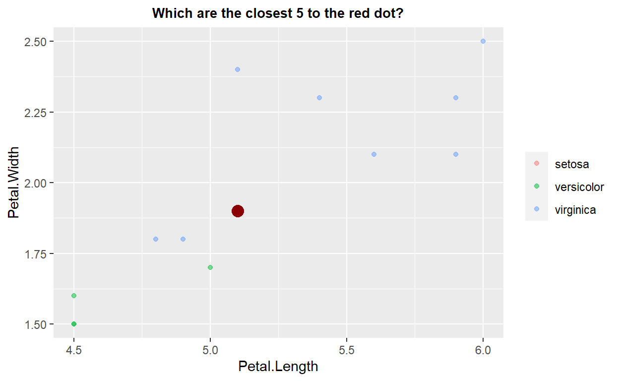
ggplot(data=graph_train,mapping = aes(x=Petal.Length,y=Petal.Width,color=Species))+geom_point(alpha=0.5) + 
   geom_point(data=graph_test, color="darkred", size=4) + theme(legend.title = element_blank())+ggtitle("Which are the closest 5 to the red dot?")+xlim(4.5,6)+ylim(1.5,2.5)+
  theme(plot.title = element_text(hjust=0.5, size=10, face='bold'))

knnModel <- train(Species ~.,
                  data = graph_train,
                  method = 'knn',
                  preProcess = c("center","scale"),
                  tuneGrid=data.frame(k=5))

predictedclass<-predict(knnModel,graph_test)

predictedclass

[1] virginica
Levels: setosa versicolor virginica

knnModel$finalModel

5-nearest neighbor model
Training set outcome distribution:

    setosa versicolor  virginica 
        10         10         10

As shown in the previous plot, when a new datum is added (e.g., the large red point), the k-nn algorithm first identifies the \(k\) nearest neighbors (in the example above this is five by default). Given these nearest neighbors, a statistical evaluation of their relevant feature is performed, and the result used to make the prediction for the new data point. The statistical evaluation can be simple, such as choosing the mode from a set of discrete classes, or more complex, such as choosing the weighted mean of the features from the nearest neighbors, where the weight might be determined by the relative distance of each neighbor from the datum of interest.

Fundamental to this algorithm is the concept of distance. To this point we have simply assumed the features used to define neighbors followed a standard Euclidean distance (i.e., normal spatial coordinates). While this is often the case, some problems require a different distance. The next subsection explores this concept in more detail.

Distance Measurements

To determine neighbors, we must adopt a definition for the distance. Naively, we might think this is simple, we adopt the common concept of distance that underlies the Pythagorean theorem: \(d = \sqrt{(x_2 - x_1)^2 + (y_2 - y_1)^2}\) where \(d\) is the distance between two-dimensional points \((x_1, y_1)\) and \((x_2, y_2)\) . However, this is really only true for data that follow a Euclidean distance metric, such as points on a cartesian plot. This is not true for calculating other distances, even spatial ones, such as the distance a plane flies on a long-distance flight. Furthermore, many data likely require an alternative definition of distance. For example, currency data, categorical data, or text data all likely require different definitions for distance.

Some of the standard distance metrics in this module include:

euclidean: supports the standard concept of spatial distance, and is the l2-norm.
manhattan: restricts distance measurements to follow grid lines. This metric is sometimes referred to as the Taxi cab distance, since taxis must follow streets, which also gives rise to its formal name, manhattan, for the street grid on the island of Manhattan. This distance is also known as the l1-norm.
haversine: calculates the distance travelled over the surface of a sphere, such as the Earth.
chebyshev: assumes the distance is equal to the greatest distance along the individual dimensions.
minkowski: a generalization of the Manhattan and Euclidean distances to arbitrary powers.

Curse of Dimensionality

In general, we strive to obtain as much data as possible to improve our model prediction. The additional data can take one of two forms: additional features, which increases the dimensionality of our data set, or additional instances, which increases the pool of data from which to draw training and testing samples. Additional instances impacts a machine learning process in a simple manner, more data requires more computational power for either storing the data, or to process the data more rapidly. Additional dimensions on the other hand, can introduce an additional complication that is known as the curse of dimensionality.

At its simplest, the curse of dimensionality relates the density of training data to the performance of our machine learning algorithm. In order to ensure sufficient density of training data across a potential sample space, the quantity of training data must increase exponentially (or very rapidly) with each new dimension. Otherwise, we end up with a space that is poorly sampled by training data.

The ‘curse of dimensionality’ is the tendency for model accuracy to initially increase as the number of variables used increases, but then reach a limit where accuracy decreases — the point where the model is overfit

Note that some algorithms are affected more strongly by the curse of dimensionality, especially techniques that rely on distance measurements. Thus, the k-nn algorithm can be strongly affected by this issue, which can be visualized by looking closely at the decision surfaces. To overcome the curse of dimensionality, one must either increase the amount of training data, or reduce the dimensionality by either identifying the most important features or deriving new features that contain most of the information.

ggplot(data=train,mapping = aes(x=Petal.Length,y=Petal.Width,color=Species))+geom_point(alpha=0.5) + 
   geom_point(data=test, color="darkred", size=1) + theme(legend.title = element_blank())+ggtitle("Knn for iris")+
  theme(plot.title = element_text(hjust=0.5, size=10, face='bold'))

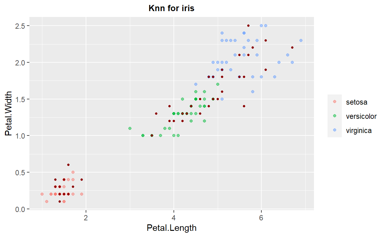
k-Nearest Neighbors: Classification

We can now apply the k-nn algorithm to the Iris data to create a classification model. The steps are demonstrated in the following code cell, where we create our estimator, fit the estimator to our training data, and generate a performance score on the testing data. Note that by default, the classification from the features of multiple neighbors is done by a simple majority vote (which is equivalent to the mode of the discrete labels). Finally, if multiple neighbors are at the same distance but have different labels, the ordering of the trading data will impact which label is used in the voting process.

set.seed(1)

indxTrain <- createDataPartition(y = iris[, names(iris) == "Species"], p = 0.7, list = F)

train <- iris[indxTrain,]
test <- iris[-indxTrain,]

# Fit the model on the training set
#set.seed(123)
knn_model_2 <- train(
  Species ~., 
  data = train, 
  method = "knn",
  trControl = trainControl("cv", number = 10),
  preProcess = c("center","scale"),
  tuneLength = 10
  )
knn_model_2

k-Nearest Neighbors 

105 samples
  4 predictor
  3 classes: 'setosa', 'versicolor', 'virginica' 

Pre-processing: centered (4), scaled (4) 
Resampling: Cross-Validated (10 fold) 
Summary of sample sizes: 94, 95, 94, 94, 95, 95, ... 
Resampling results across tuning parameters:

  k   Accuracy   Kappa    
   5  0.9525758  0.9278883
   7  0.9525758  0.9278883
   9  0.9425758  0.9127368
  11  0.9425758  0.9127368
  13  0.9516667  0.9266608
  15  0.9525758  0.9282321
  17  0.9525758  0.9282321
  19  0.9425758  0.9130806
  21  0.9425758  0.9130806
  23  0.9125758  0.8671529

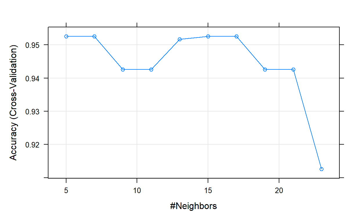
Accuracy was used to select the optimal model using the
 largest value.
The final value used for the model was k = 17.

# Plot model error vs different values of k
plot(knn_model_2)

# Best tuning parameter k that minimize the error
knn_model_2$bestTune

   k
7 17

# Make predictions on the test data
predictions <- predict(knn_model_2,test)
head(predictions)

[1] setosa setosa setosa setosa setosa setosa
Levels: setosa versicolor virginica

# Compute the prediction error 
confusionMatrix(predictions, test$Species)

Confusion Matrix and Statistics

            Reference
Prediction   setosa versicolor virginica
  setosa         15          0         0
  versicolor      0         14         2
  virginica       0          1        13

Overall Statistics
                                         
               Accuracy : 0.9333         
                 95% CI : (0.8173, 0.986)
    No Information Rate : 0.3333         
    P-Value [Acc > NIR] : < 2.2e-16      
                                         
                  Kappa : 0.9            
                                         
 Mcnemar's Test P-Value : NA             

Statistics by Class:

                     Class: setosa Class: versicolor Class: virginica
Sensitivity                 1.0000            0.9333           0.8667
Specificity                 1.0000            0.9333           0.9667
Pos Pred Value              1.0000            0.8750           0.9286
Neg Pred Value              1.0000            0.9655           0.9355
Prevalence                  0.3333            0.3333           0.3333
Detection Rate              0.3333            0.3111           0.2889
Detection Prevalence        0.3333            0.3556           0.3111
Balanced Accuracy           1.0000            0.9333           0.9167

Exercise 1

Use the code chunk above and answer the following questions.

Change the data split size from 70/30 to 50/50. How does that effect the results?
What was the optimal number of neighbors from number 1? Why do you think that is?
Change the 10 to 5 in trainControl("cv", number = 10) and the 10 to 20 in tuneLength = 10. How did that change the results?

Performance Metrics

In our Iris data classification example, we are performing a multiple classification task where we have more than two labels. As a result, one of the simplest ways to understand our performance is to create and display a confusion matrix. A confusion matrix has rows that correspond to the true labels and columns that correspond to the predicted labels. The elements of the confusion matrix contain the number of instances with true label given by the row index and the predicted label by the column index. A perfect classification, therefore, would have a confusion matrix populated entirely along the diagonal.

# Compute the prediction error 
confusionMatrix(predictions, test$Species)

Confusion Matrix and Statistics

            Reference
Prediction   setosa versicolor virginica
  setosa         15          0         0
  versicolor      0         14         2
  virginica       0          1        13

Overall Statistics
                                         
               Accuracy : 0.9333         
                 95% CI : (0.8173, 0.986)
    No Information Rate : 0.3333         
    P-Value [Acc > NIR] : < 2.2e-16      
                                         
                  Kappa : 0.9            
                                         
 Mcnemar's Test P-Value : NA             

Statistics by Class:

                     Class: setosa Class: versicolor Class: virginica
Sensitivity                 1.0000            0.9333           0.8667
Specificity                 1.0000            0.9333           0.9667
Pos Pred Value              1.0000            0.8750           0.9286
Neg Pred Value              1.0000            0.9655           0.9355
Prevalence                  0.3333            0.3333           0.3333
Detection Rate              0.3333            0.3111           0.2889
Detection Prevalence        0.3333            0.3556           0.3111
Balanced Accuracy           1.0000            0.9333           0.9167

While the confusion matrix provides a useful visualization of the performance of a classification, in some cases a numerical score is desired. A number of different scores have been proposed for classification tasks, which one is most useful often depends on the nature of the classification task. Two commonly used scores are the precision and the recall. Note that both of these scores are ratios, and thus take values between zero (bad) and one (good).

Simply put, the precision (sometimes called the positive predictive value) is a measure of how many instances were correctly classified with the appropriate label. Thus, the precision is computed as the ratio of the number of instances correctly classified with a given label to the number of instances that actually have that label. Recall (sometimes called sensitivity) measures how many of the instances that were classified with a given label actually have that label. Thus, recall is computed as the ratio of correctly classified instances of a given label to the number of instances classified with that label.

To generate one single numerical score, the f1-score was created, which is simply the harmonic mean of the precision and the recall (note, we must use the harmonic mean since these scores are actually ratios). Finally, one additional value of interest when interpreting these results is the support, which is the number of instances of each label in the testing set that was used to compute the indicated score.

k-Nearest Neighbors: Hyperparameters

Machine learning algorithms often have tuning parameters that are extrinsic to the algorithm that cannot be determined directly from the data being analyzed. These parameters are formally known as hyperparameters. The k-nn algorithm has two hyperparameters: the number of nearest neighbors and a weighting scheme. To demonstrate how these hyperparameters affect the performance of the k-nn algorithm the following two subsections create a k-nn estimator with different values for these hyperparameters and display the results. To more effectively visualize the impact of these hyperparameters, we introduce the decision surface.

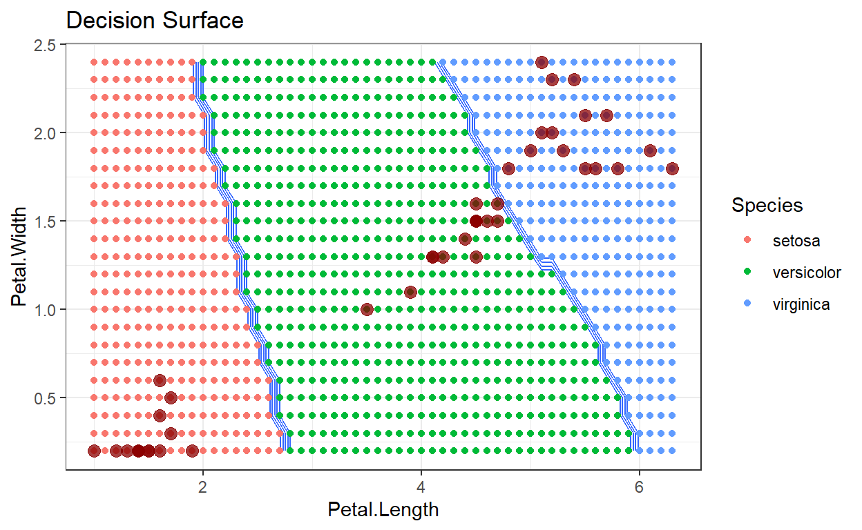
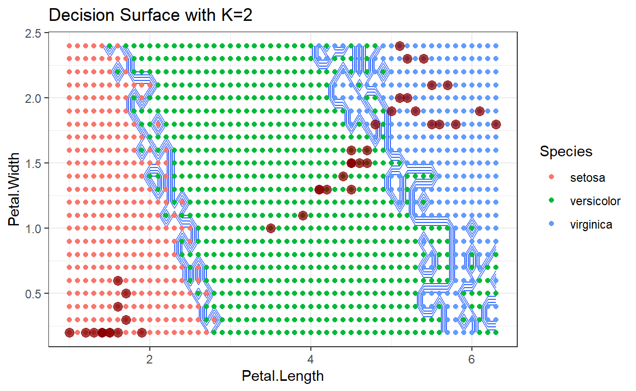
A decision surface is a visualization that shows a particular space occupied by the training data, in this case just the two dimensions: Sepal Width and Petal Width. The training data, color coded by their class, are displayed on this plot. In addition, the entire space spanned by the plot has been divided into a mesh grid, and each point in the mesh grid has been classified by the algorithm being analyzed. This has the effect of showing how new test data points would be classified as they move around the plot region. By comparing decision surfaces that correspond to different hyperparameter values, we can understand the corresponding change in the algorithm’s performance.

library(caret) 
data(iris)

indxTrain <- createDataPartition(y = iris[, names(iris) == "Species"], p = 0.7, list = F)

train <- iris[indxTrain,]
test <- iris[-indxTrain,]

knnModel <- train(Species ~.,
                  data = train,
                  method = 'knn')

pl = seq(min(test$Petal.Length), max(test$Petal.Length), by=0.1)
pw = seq(min(test$Petal.Width), max(test$Petal.Width), by=0.1)

# generates the boundaries for your graph
lgrid <- expand.grid(Petal.Length=pl, 
                     Petal.Width=pw,
                     Sepal.Length = 5.4,
                     Sepal.Width=3.1)

knnPredGrid <- predict(knnModel, newdata=lgrid)
knnPredGrid = as.numeric(knnPredGrid)

# get the points from the test data...
testPred <- predict(knnModel, newdata=test)
testPred <- as.numeric(testPred)
# this gets the points for the testPred...
test$Pred <- testPred

probs <- matrix(knnPredGrid, length(pl), length(pw))

ggplot(data=lgrid) + stat_contour(aes(x=Petal.Length, y=Petal.Width, z=knnPredGrid),bins=10) +
  geom_point(aes(x=Petal.Length, y=Petal.Width, colour=as.factor(knnPredGrid)))+
  geom_point(data=test, aes(x=Petal.Length, y=Petal.Width), size=3, alpha=0.75, color="darkred")+
  theme_bw()+ 
  labs(color = "Species")+
  ggtitle("Decision Surface")+
  scale_color_hue(labels=c('setosa', 'versicolor', 'virginica'))

Decision surface with k=2

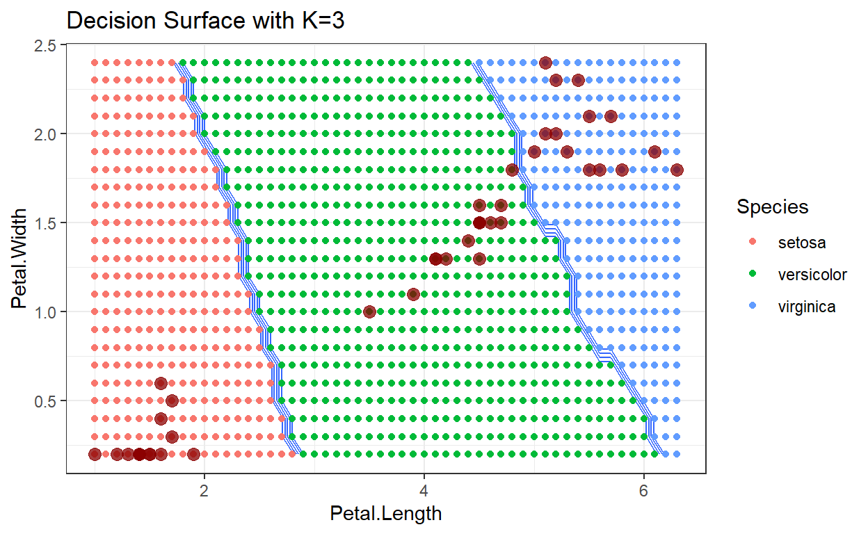
Decision surface with k=3

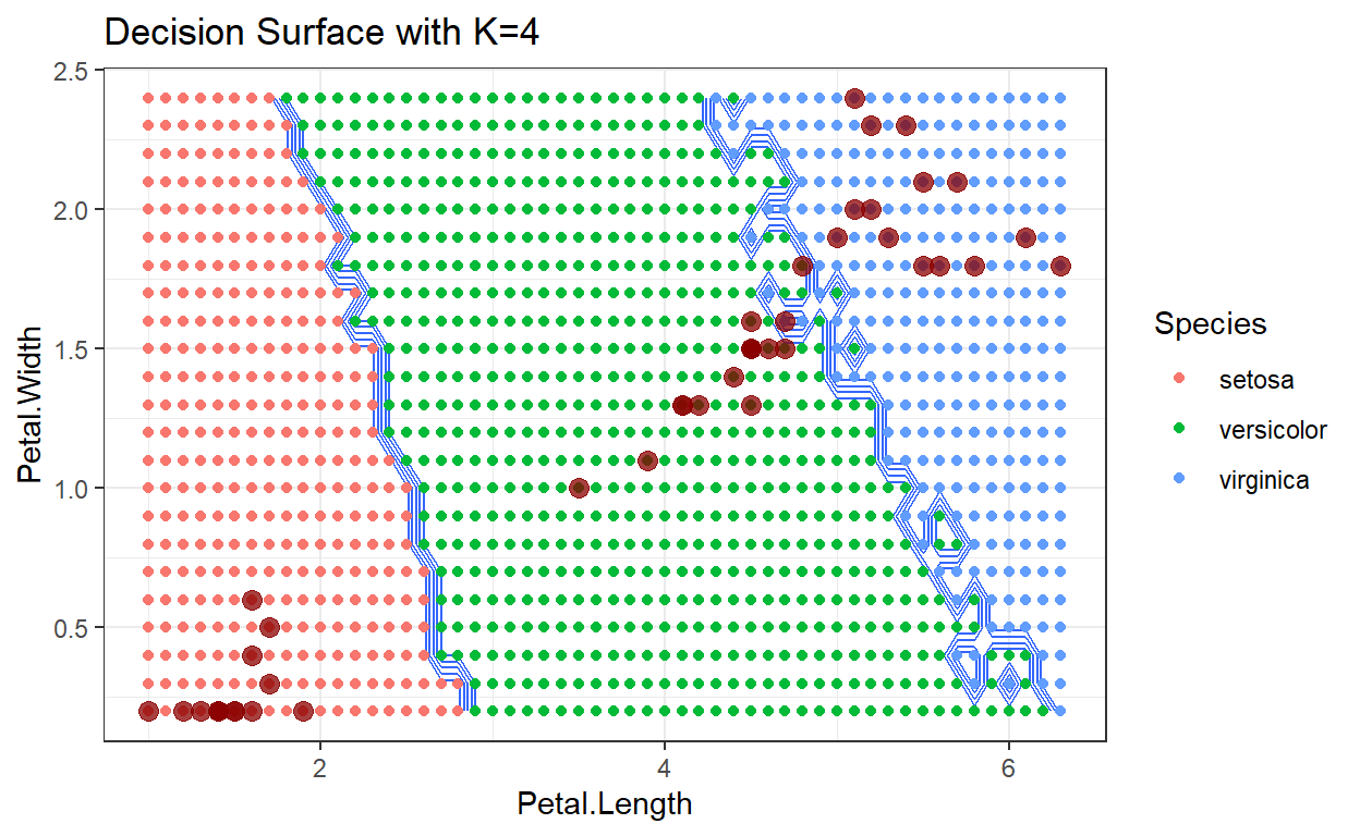
Decision surface with k=4

Neighbors

As the number of neighbors increases, we tend to average over the distribution of training data, which makes the decision surface cleaner with smaller variations. Depending on the data being analyzed, this can be either a good or bad result.

Weights

The second hyperparameter that can be specified in the k-nn algorithm is the weight used to compute the statistical summary of the neighbor features. By default each neighbor is treated equally. The other simple choice for the weight hyperparameter is to use distance weighting, where the features from different neighbors are weighted by the inverse of their distance. Thus, closer points are weighted more than distant neighbors. Finally, the third option for this hyperparameter is to provide a user-defined function that accepts an array of distances and returns the appropriate weights. This last option enables an analyst to leverage one of the other distance metrics discussed.

k-Nearest Neighbors: Regression

As is the case with many of the supervised learning algorithms the k-nn algorithm can be used for classification (as demonstrated previously) and for regression.

set.seed(1)

indxTrain <- createDataPartition(y = iris[, names(iris) == "Sepal.Width"], p = 0.7, list = F)

train <- iris[indxTrain,]
test <- iris[-indxTrain,]

# Fit the model on the training set
#set.seed(123)
knn_model_3 <- train(
  Sepal.Width ~., 
  data = train, 
  method = "knn",
  trControl = trainControl("cv", number = 10),
  preProcess = c("center","scale"),
  tuneLength = 10
  )
knn_model_3

k-Nearest Neighbors 

106 samples
  4 predictor

Pre-processing: centered (5), scaled (5) 
Resampling: Cross-Validated (10 fold) 
Summary of sample sizes: 94, 97, 95, 96, 96, 96, ... 
Resampling results across tuning parameters:

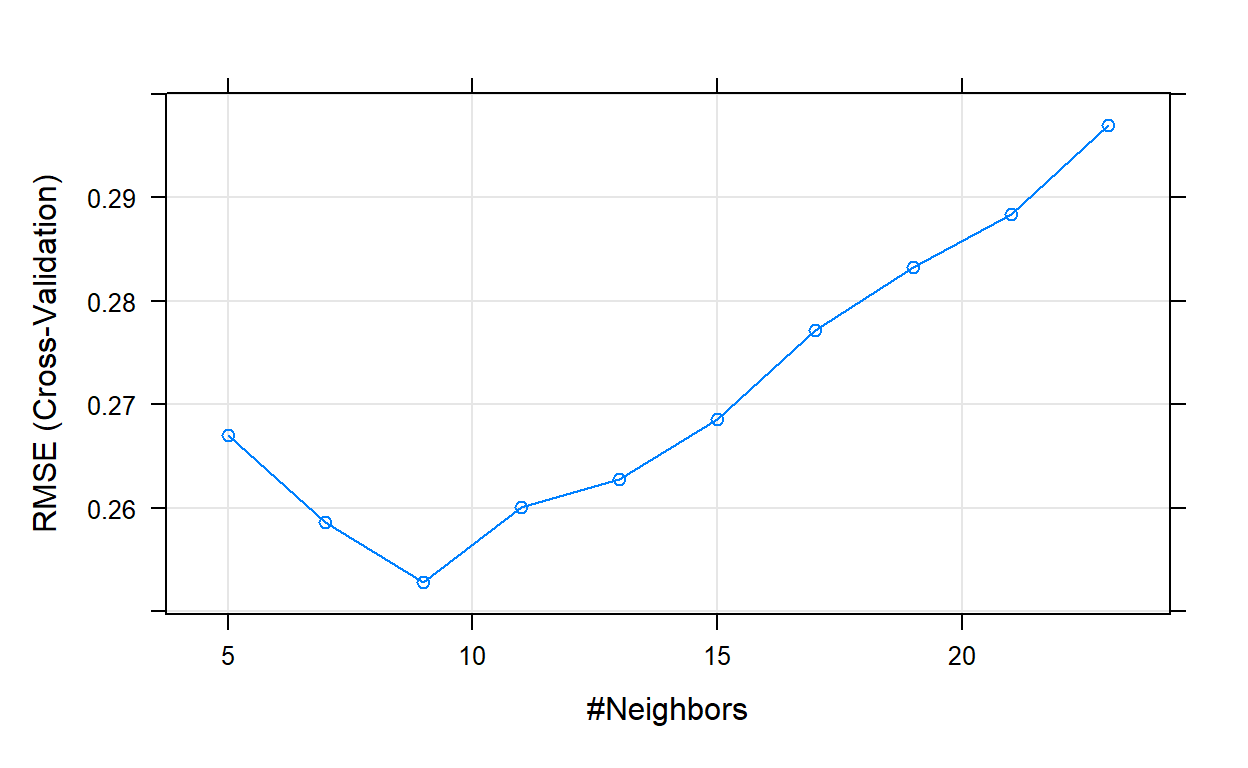
  k   RMSE       Rsquared   MAE      
   5  0.2670473  0.6263350  0.2136713
   7  0.2585939  0.6670098  0.2062614
   9  0.2528080  0.6790589  0.2043737
  11  0.2600811  0.6723692  0.2054493
  13  0.2627914  0.6695809  0.2055432
  15  0.2685241  0.6648964  0.2099648
  17  0.2771452  0.6535122  0.2166236
  19  0.2832965  0.6448399  0.2218299
  21  0.2883884  0.6240123  0.2252297
  23  0.2969795  0.6006586  0.2305546

RMSE was used to select the optimal model using the smallest value.
The final value used for the model was k = 9.

# Plot model error vs different values of k
plot(knn_model_3)

# Best tuning parameter k that minimize the error
knn_model_3$bestTune

  k
3 9

# Make predictions on the test data
predictions <- predict(knn_model_3,test)
head(predictions)

[1] 3.011111 3.811111 3.077778 3.233333 3.722222 3.070000

# Compute the prediction error 
RMSE(predictions, test$Sepal.Width)

[1] 0.2983394

Exercise 2