Dimensionality Reduction

When confronted with a large, multi-dimensional data set, one approach to simplify any subsequent analysis is to reduce the number of dimensions (or features) that must be processed. In some cases, features can be removed from an analysis based on business logic, or the features that contain the most information can be quantified somehow. More generally, however, we can employ dimensional reduction, a machine learning technique that quantifies relationships between the original dimensions (or features, attributes, or columns of a DataFrame) to identify new dimensions that better capture the inherent relationships within the data.

PCA

The standard technique to perform this is known as principal component analysis, or PCA. Mathematically, we can derive PCA by using linear algebra to solve a set of linear equations. This process effectively rotates the data into a new set of dimensions, and by ranking the importance of the new dimensions, we can optimally select fewer dimensions for use in other machine learning algorithms.

The PCA estimator requires one tunable hyper-parameter that specifies the target number of dimensions. This value can be arbitrarily selected, perhaps based on prior information, or it can be iteratively determined. After the model is created, we fit the model to the data and next create our new, rotated data set. This is demonstrated in the next code cell.

library(caret)
#store our data in another object
dat <- iris
#take the 4 continuous variables and perform PCA
caret.pca <- preProcess(dat[,-5], method="pca",pcaComp=2)

caret.pca

Created from 150 samples and 4 variables

Pre-processing:
  - centered (4)
  - ignored (0)
  - principal component signal extraction (4)
  - scaled (4)

PCA used 2 components as specified

caret.pca$
#use that data to form our new inputs
dat2 <- predict(caret.pca, dat[,-5])


#using stats
stat.pca <- prcomp(dat[,-5],
                 center = TRUE,
                 scale. = TRUE) 

# plot method
plot(stat.pca, type = "l")

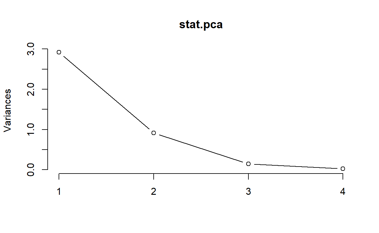
summary(stat.pca)

Importance of components:
                          PC1    PC2     PC3     PC4
Standard deviation     1.7084 0.9560 0.38309 0.14393
Proportion of Variance 0.7296 0.2285 0.03669 0.00518
Cumulative Proportion  0.7296 0.9581 0.99482 1.00000

Below is a graphical representation¹

At the end of the previous code cell, we measure the amount of the original variance (or spread) in the original data that is captured by each new dimension. As this example shows, these two new dimensions capture almost 96% of the variance in the original data. This means that any analysis that uses only these two new dimensions will closely represent the analysis if performed on the entire data.

Clustering

The last machine learning technique we will explore in this notebook is cluster finding. In this introductory notebook, we will demonstrate one of the simplest clustering techniques, spatial clustering, which seeks to first find NN clusters in a data set and to subsequently identify to which cluster each instance (or data point) belongs. The specific algorithm we employ below is the k-means algorithm, which is one of the simplest to understand. In this algorithm, we start with a guess for the number of clusters (again this can be based on prior information or iteratively quantified). We randomly place cluster centers in the data and determine how well the data cluster to these cluster centers. This information is used to pick new cluster centers, and the process continues until a solution converges (or we reach a predefined number of iterations).

#lets split the data 60/40
library(caret)
trainIndex <- createDataPartition(iris$Species, p = .6, list = FALSE, times = 1)

#grab the data
irisTrain <- iris[ trainIndex,]
irisTest  <- iris[-trainIndex,]

#normalize variables
preProcValues <- preProcess(irisTrain, method = c("center", "scale"))
trainTransformed <- predict(preProcValues, irisTrain)

preProcValues <- preProcess(irisTest, method = c("center", "scale"))
testTransformed <- predict(preProcValues, irisTest)

#cluster
Clusters<-kmeans(trainTransformed[,-5],centers=3)

Clusters

K-means clustering with 3 clusters of sizes 35, 26, 29

Cluster means:
  Sepal.Length Sepal.Width Petal.Length Petal.Width
1    1.0056523 -0.02989108    0.9341394  0.98620899
2   -0.2415149 -0.99086060    0.1708722  0.04873749
3   -0.9971877  0.92443323   -1.2806054 -1.23394791

Clustering vector:
  1   2   6   7   9  10  11  14  16  18  21  22  23  25  27  28  29 
  3   3   3   3   3   3   3   3   3   3   3   3   3   3   3   3   3 
 30  31  32  33  35  36  42  44  45  46  47  49  50  53  55  56  57 
  3   3   3   3   3   3   2   3   3   3   3   3   3   1   1   2   1 
 58  60  64  65  66  68  70  71  74  75  76  77  81  82  83  85  87 
  2   2   2   2   1   2   2   1   2   2   1   1   2   2   2   2   1 
 88  91  93  94  95  97  98  99 100 102 103 104 105 106 108 109 110 
  2   2   2   2   2   2   2   2   2   2   1   1   1   1   1   1   1 
112 116 117 119 120 121 123 127 128 132 134 135 137 138 139 140 141 
  1   1   1   1   2   1   1   1   1   1   1   2   1   1   1   1   1 
142 144 145 146 150 
  1   1   1   1   1 

Within cluster sum of squares by cluster:
[1] 36.01159 22.84438 23.93414
 (between_SS / total_SS =  76.7 %)

Available components:

[1] "cluster"      "centers"      "totss"        "withinss"    
[5] "tot.withinss" "betweenss"    "size"         "iter"        
[9] "ifault"

The above list is an output of the kmeans() function. Let’s see some of the important ones closely:

cluster: a vector of integers (from 1:k) indicating the cluster to which each point is allocated.
centers: a matrix of cluster centers.
withinss: vector of within-cluster sum of squares, one component per cluster.
tot.withinss: total within-cluster sum of squares. That is, sum(withinss).
size: the number of points in each cluster.

library(tidyverse)

Clusterdata<-trainTransformed
Clusterdata$Cluster<-as.factor(Clusters$cluster)

#view the whole dataset
knitr::kable(Clusterdata)%>%
  kableExtra::kable_styling("striped")%>%
  kableExtra::scroll_box(width = "100%",height="300px")

	Sepal.Length	Sepal.Width	Petal.Length	Petal.Width	Species	Cluster
1	-0.8947930	1.0461878	-1.3310527	-1.3067741	setosa	3
2	-1.1323487	-0.1307735	-1.3310527	-1.3067741	setosa	3
6	-0.5384595	1.9877569	-1.1622484	-1.0427793	setosa	3
7	-1.4886822	0.8107956	-1.3310527	-1.1747767	setosa	3
9	-1.7262378	-0.3661657	-1.3310527	-1.3067741	setosa	3
10	-1.1323487	0.1046188	-1.2747846	-1.4387714	setosa	3
11	-0.5384595	1.5169724	-1.2747846	-1.3067741	setosa	3
14	-1.8450156	-0.1307735	-1.4998569	-1.4387714	setosa	3
16	-0.1821260	3.1647182	-1.2747846	-1.0427793	setosa	3
18	-0.8947930	1.0461878	-1.3310527	-1.1747767	setosa	3
21	-0.5384595	0.8107956	-1.1622484	-1.3067741	setosa	3
22	-0.8947930	1.5169724	-1.2747846	-1.0427793	setosa	3
23	-1.4886822	1.2815801	-1.5561250	-1.3067741	setosa	3
25	-1.2511265	0.8107956	-1.0497123	-1.3067741	setosa	3
27	-1.0135708	0.8107956	-1.2185165	-1.0427793	setosa	3
28	-0.7760152	1.0461878	-1.2747846	-1.3067741	setosa	3
29	-0.7760152	0.8107956	-1.3310527	-1.3067741	setosa	3
30	-1.3699043	0.3400110	-1.2185165	-1.3067741	setosa	3
31	-1.2511265	0.1046188	-1.2185165	-1.3067741	setosa	3
32	-0.5384595	0.8107956	-1.2747846	-1.0427793	setosa	3
33	-0.7760152	2.4585414	-1.2747846	-1.4387714	setosa	3
35	-1.1323487	0.1046188	-1.2747846	-1.3067741	setosa	3
36	-1.0135708	0.3400110	-1.4435888	-1.3067741	setosa	3
42	-1.6074600	-1.7785193	-1.3873208	-1.1747767	setosa	2
44	-1.0135708	1.0461878	-1.2185165	-0.7787845	setosa	3
45	-0.8947930	1.7523646	-1.0497123	-1.0427793	setosa	3
46	-1.2511265	-0.1307735	-1.3310527	-1.1747767	setosa	3
47	-0.8947930	1.7523646	-1.2185165	-1.3067741	setosa	3
49	-0.6572373	1.5169724	-1.2747846	-1.3067741	setosa	3
50	-1.0135708	0.5754033	-1.3310527	-1.3067741	setosa	3
53	1.2432080	0.1046188	0.6383301	0.4091919	versicolor	1
55	0.7680966	-0.6015580	0.4695259	0.4091919	versicolor	1
56	-0.1821260	-0.6015580	0.4132578	0.1451971	versicolor	2
57	0.5305410	0.5754033	0.5257939	0.5411893	versicolor	1
58	-1.1323487	-1.5431271	-0.2619592	-0.2507950	versicolor	2
60	-0.7760152	-0.8369503	0.0756493	0.2771945	versicolor	2
64	0.2929853	-0.3661657	0.5257939	0.2771945	versicolor	2
65	-0.3009038	-0.3661657	-0.0931549	0.1451971	versicolor	2
66	1.0056523	0.1046188	0.3569897	0.2771945	versicolor	1
68	-0.0633482	-0.8369503	0.1881855	-0.2507950	versicolor	2
70	-0.3009038	-1.3077348	0.0756493	-0.1187976	versicolor	2
71	0.0554297	0.3400110	0.5820620	0.8051840	versicolor	1
74	0.2929853	-0.6015580	0.5257939	0.0131997	versicolor	2
75	0.6493188	-0.3661657	0.3007216	0.1451971	versicolor	2
76	0.8868745	-0.1307735	0.3569897	0.2771945	versicolor	1
77	1.1244301	-0.6015580	0.5820620	0.2771945	versicolor	1
81	-0.4196817	-1.5431271	0.0193812	-0.1187976	versicolor	2
82	-0.4196817	-1.5431271	-0.0368869	-0.2507950	versicolor	2
83	-0.0633482	-0.8369503	0.0756493	0.0131997	versicolor	2
85	-0.5384595	-0.1307735	0.4132578	0.4091919	versicolor	2
87	1.0056523	0.1046188	0.5257939	0.4091919	versicolor	1
88	0.5305410	-1.7785193	0.3569897	0.1451971	versicolor	2
91	-0.4196817	-1.0723425	0.3569897	0.0131997	versicolor	2
93	-0.0633482	-1.0723425	0.1319174	0.0131997	versicolor	2
94	-1.0135708	-1.7785193	-0.2619592	-0.2507950	versicolor	2
95	-0.3009038	-0.8369503	0.2444535	0.1451971	versicolor	2
97	-0.1821260	-0.3661657	0.2444535	0.1451971	versicolor	2
98	0.4117631	-0.3661657	0.3007216	0.1451971	versicolor	2
99	-0.8947930	-1.3077348	-0.4307634	-0.1187976	versicolor	2
100	-0.1821260	-0.6015580	0.1881855	0.1451971	versicolor	2
102	-0.0633482	-0.8369503	0.7508663	0.9371814	virginica	2
103	1.4807636	-0.1307735	1.2010109	1.2011761	virginica	1
104	0.5305410	-0.3661657	1.0322067	0.8051840	virginica	1
105	0.7680966	-0.1307735	1.1447428	1.3331735	virginica	1
106	2.0746528	-0.1307735	1.5948874	1.2011761	virginica	1
108	1.7183193	-0.3661657	1.4260832	0.8051840	virginica	1
109	1.0056523	-1.3077348	1.1447428	0.8051840	virginica	1
110	1.5995415	1.2815801	1.3135471	1.7291657	virginica	1
112	0.6493188	-0.8369503	0.8634024	0.9371814	virginica	1
116	0.6493188	0.3400110	0.8634024	1.4651709	virginica	1
117	0.7680966	-0.1307735	0.9759386	0.8051840	virginica	1
119	2.1934306	-1.0723425	1.7636917	1.4651709	virginica	1
120	0.1742075	-2.0139116	0.6945982	0.4091919	virginica	2
121	1.2432080	0.3400110	1.0884747	1.4651709	virginica	1
123	2.1934306	-0.6015580	1.6511555	1.0691788	virginica	1
127	0.4117631	-0.6015580	0.5820620	0.8051840	virginica	1
128	0.2929853	-0.1307735	0.6383301	0.8051840	virginica	1
132	2.4309863	1.7523646	1.4823513	1.0691788	virginica	1
134	0.5305410	-0.6015580	0.7508663	0.4091919	virginica	1
135	0.2929853	-1.0723425	1.0322067	0.2771945	virginica	2
137	0.5305410	0.8107956	1.0322067	1.5971683	virginica	1
138	0.6493188	0.1046188	0.9759386	0.8051840	virginica	1
139	0.1742075	-0.1307735	0.5820620	0.8051840	virginica	1
140	1.2432080	0.1046188	0.9196705	1.2011761	virginica	1
141	1.0056523	0.1046188	1.0322067	1.5971683	virginica	1
142	1.2432080	0.1046188	0.7508663	1.4651709	virginica	1
144	1.1244301	0.3400110	1.2010109	1.4651709	virginica	1
145	1.0056523	0.5754033	1.0884747	1.7291657	virginica	1
146	1.0056523	-0.1307735	0.8071343	1.4651709	virginica	1
150	0.0554297	-0.1307735	0.7508663	0.8051840	virginica	1

#Remember me
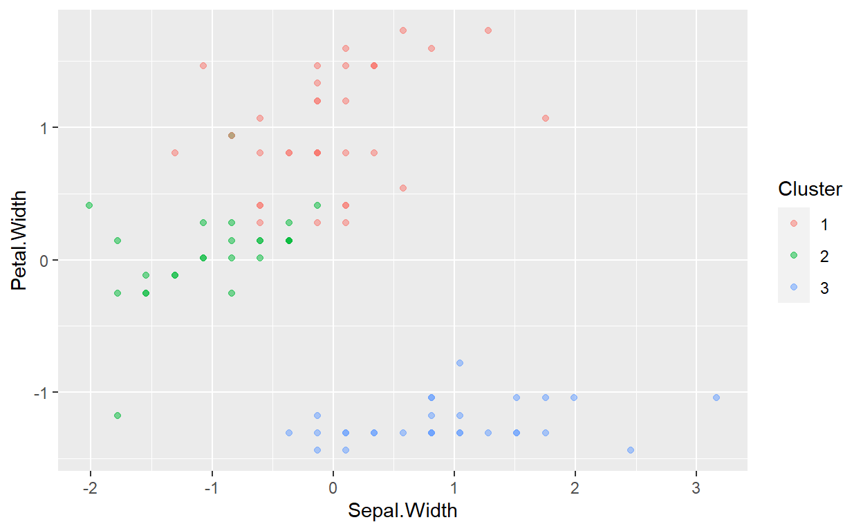
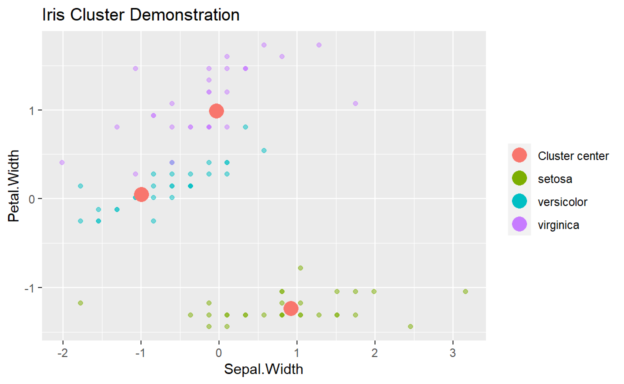
ggplot(data=Clusterdata,mapping = aes(x=Sepal.Width,y=Petal.Width,color=Cluster))+geom_point(alpha=0.5)

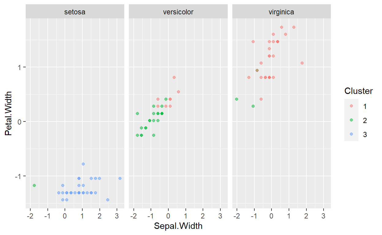
ggplot(data=Clusterdata,mapping = aes(x=Sepal.Width,y=Petal.Width,color=Cluster))+geom_point(alpha=0.5)+facet_wrap(~Species)

ggplot(data=Clusterdata,mapping = aes(x=Sepal.Width,y=Petal.Width,color=Species))+
  geom_point(alpha=0.5) + 
   geom_point(data=as.data.frame(Clusters$centers), aes(color="Cluster center"), size=5) + 
  theme(legend.title = element_blank())+ggtitle("Iris Cluster Demonstration")

Exercise 1

Using the code above, answer the following question.

Change the pcaComp hyper-parameter in the PCA code example to three (and four) in the Dimensionality Reduction section. What are the new explained variances?

Answer

Explanation For the first code chunk: First let me apologize for not doing this initially. I did not have it added in because you have to do the calculations by hand, but here they are…This is using 2 principal components and then calculating the proportion of variance explained by each component. I use an apply function and do it the long way. This sets us up to try the of number of components

For the second code chunk: Change the number of components to 3.

For the third code chunk: Change the number of components to 4.

Code

First Code Chunk

library(caret)
#store our data in another object
dat <- iris
#take the 4 continuous variables and perform PCA
caret.pca <- preProcess(dat[,-5], method="pca",pcaComp=2)

caret.pca

Created from 150 samples and 4 variables

Pre-processing:
  - centered (4)
  - ignored (0)
  - principal component signal extraction (4)
  - scaled (4)

PCA used 2 components as specified

#use that data to form our new inputs
dat2 <- predict(caret.pca, dat[,-5])

#apply runs a loop for you
#dat2 is the data
#the 2 tells it to run the loop over the columns (1 is rows)
#sd is the function for standard deviation
#^2 squares it so we can find variance
#sum adds them to get total variance
Components2<-apply(dat2,2,sd)^2/sum((apply(dat2,2,sd))^2)

Components2

      PC1       PC2 
0.7615072 0.2384928

#doing the above by hand
sd(dat2$PC1)^2/(sd(dat2$PC1)^2+sd(dat2$PC2)^2)

[1] 0.7615072

sd(dat2$PC2)^2/(sd(dat2$PC1)^2+sd(dat2$PC2)^2)

[1] 0.2384928

Second Code Chunk

library(caret)
#store our data in another object
dat <- iris
#take the 4 continuous variables and perform PCA
caret.pca <- preProcess(dat[,-5], method="pca",pcaComp=3)

caret.pca

Created from 150 samples and 4 variables

Pre-processing:
  - centered (4)
  - ignored (0)
  - principal component signal extraction (4)
  - scaled (4)

PCA used 3 components as specified

#use that data to form our new inputs
dat2 <- predict(caret.pca, dat[,-5])

#apply runs a loop for you
#dat2 is the data
#the 2 tells it to run the loop over the columns (1 is rows)
#sd is the function for standard deviation
#^2 squares it so we can find variance
#sum adds them to get total variance
Components3<-apply(dat2,2,sd)^2/sum((apply(dat2,2,sd))^2)

Components3

       PC1        PC2        PC3 
0.73342264 0.22969715 0.03688021

Third Code Chunk

library(caret)
#store our data in another object
dat <- iris
#take the 4 continuous variables and perform PCA
caret.pca <- preProcess(dat[,-5], method="pca",pcaComp=4)

caret.pca

Created from 150 samples and 4 variables

Pre-processing:
  - centered (4)
  - ignored (0)
  - principal component signal extraction (4)
  - scaled (4)

PCA used 4 components as specified

#use that data to form our new inputs
dat2 <- predict(caret.pca, dat[,-5])

#apply runs a loop for you
#dat2 is the data
#the 2 tells it to run the loop over the columns (1 is rows)
#sd is the function for standard deviation
#^2 squares it so we can find variance
#sum adds them to get total variance
Components4<-apply(dat2,2,sd)^2/sum((apply(dat2,2,sd))^2)

Components4

        PC1         PC2         PC3         PC4 
0.729624454 0.228507618 0.036689219 0.005178709

Answer

By comparing the variances we see that as the number of components increase each individual component’s explained variance drops.

Components2

      PC1       PC2 
0.7615072 0.2384928

Components3

       PC1        PC2        PC3 
0.73342264 0.22969715 0.03688021

Components4

        PC1         PC2         PC3         PC4 
0.729624454 0.228507618 0.036689219 0.005178709

Change the `centers` hyper-parameter in the cluster finding code example to two (and four) in the Clustering section. Where are the new cluster centers? Does this look better or worse?
What does the set.seed function in R do? Why use it? Should we have used it above?

https://www.r-bloggers.com/2013/11/computing-and-visualizing-pca-in-r/↩︎