Time to blow RSquared up¹ 💥

R-squared is a statistic that often accompanies regression output. It ranges in value from 0 to 1 and is usually interpreted as summarizing the percent of variation in the response that the regression model explains. So an R-squared of 0.65 might mean that the model explains about 65% of the variation in our dependent variable. Given this logic, we prefer our regression models have a high R-squared.

In R, we typically get R-squared by calling the summary function on a model object. Here’s a quick example using simulated data:

# independent variable
x <- 1:20 
# for reproducibility
set.seed(1) 
# dependent variable; function of x with random error
y <- 2 + 0.5*x + rnorm(20,0,3) 
# simple linear regression
mod <- lm(y~x)
# request just the r-squared value
summary(mod)$r.squared

[1] 0.6026682

One way to express R-squared is as the sum of squared fitted-value deviations divided by the sum of squared original-value deviations:

\[ R^{2} = \frac{\sum (\hat{y} – \bar{\hat{y}})^{2}}{\sum (y – \bar{y})^{2}} \]

We can calculate it directly using our model object like so:

# extract fitted (or predicted) values from model
f <- mod$fitted.values
# sum of squared fitted-value deviations
mss <- sum((f - mean(f))^2)
# sum of squared original-value deviations
tss <- sum((y - mean(y))^2)
# r-squared
mss/tss

[1] 0.6026682

1. R-squared does not measure goodness of fit. It can be arbitrarily low when the model is completely correct. By making\(σ^2\) large, we drive R-squared towards 0, even when every assumption of the simple linear regression model is correct in every particular.

What is \(σ^2\)? When we perform linear regression, we assume our model almost predicts our dependent variable. The difference between “almost” and “exact” is assumed to be a draw from a Normal distribution with mean 0 and some variance we call \(σ^2\).

This statement is easy enough to demonstrate. The way we do it here is to create a function that (1) generates data meeting the assumptions of simple linear regression (independent observations, normally distributed errors with constant variance), (2) fits a simple linear model to the data, and (3) reports the R-squared. Notice the only parameter for sake of simplicity is sigma. We then “apply” this function to a series of increasing \(σ\) values and plot the results.

r2.0 <- function(sig){
  # our predictor
  x <- seq(1,10,length.out = 100)   
  # our response; a function of x plus some random noise
  y <- 2 + 1.2*x + rnorm(100,0,sd = sig) 
  # print the R-squared value
  summary(lm(y ~ x))$r.squared          
}

sigmas <- seq(0.5,20,length.out = 20)
 # apply our function to a series of sigma values
rout <- sapply(sigmas, r2.0)            
plot(rout ~ sigmas, type="b")

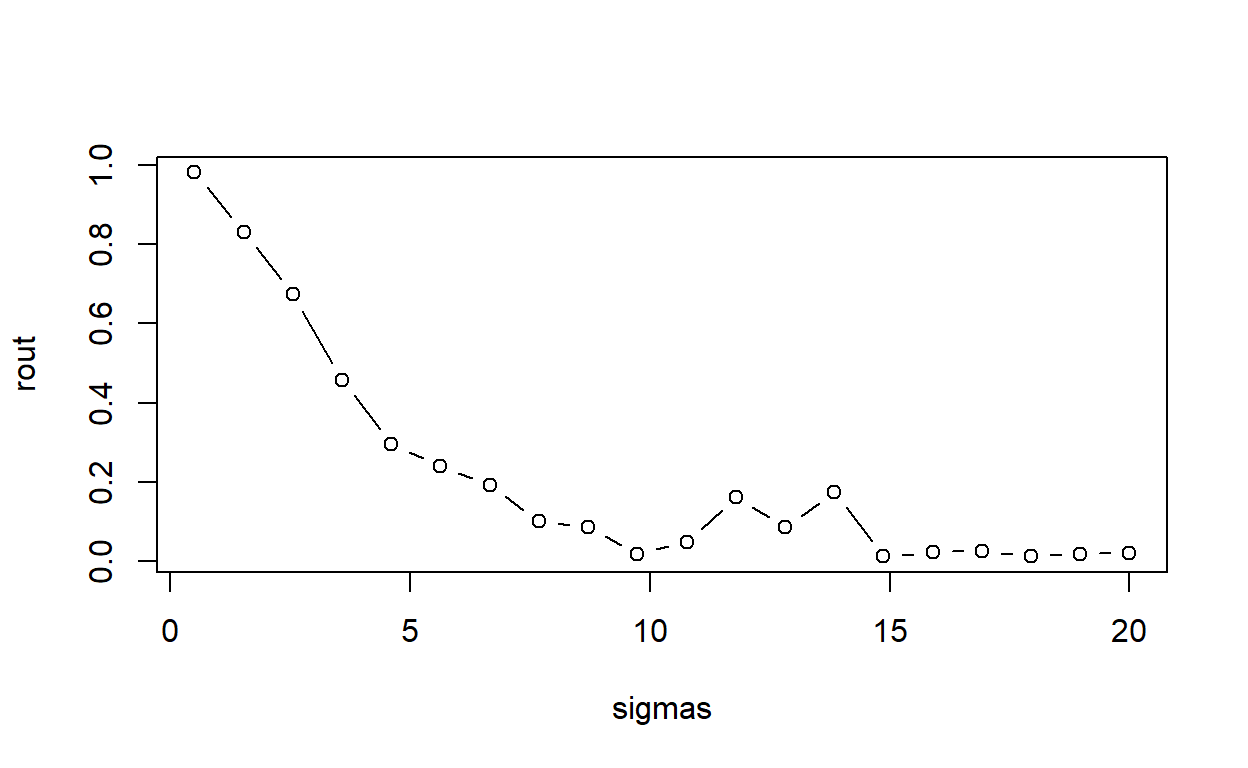
R-squared tanks hard with increasing sigma, even though the model is completely correct in every respect.

R-squared can be arbitrarily close to 1 when the model is totally wrong.

The point being made is that R-squared does not measure goodness of fit.

set.seed(1)
# our predictor is data from an exponential distribution
x <- rexp(50,rate=0.005)
# non-linear data generation
y <- (x-1)^2 * runif(50, min=0.8, max=1.2) 
# clearly non-linear
plot(x,y)

summary(lm(y ~ x))$r.squared

[1] 0.8485146

It’s very high at about 0.85, but the model is completely wrong. Using R-squared to justify the “goodness” of our model in this instance would be a mistake. Hopefully one would plot the data first and recognize that a simple linear regression in this case would be inappropriate.

3. R-squared says nothing about prediction error, even with \(σ^2\) exactly the same, and no change in the coefficients. R-squared can be anywhere between 0 and 1 just by changing the range of X. We’re better off using Mean Square Error (MSE) as a measure of prediction error.

MSE is basically the fitted y values minus the observed y values, squared, then summed, and then divided by the number of observations.

Let’s demonstrate this statement by first generating data that meets all simple linear regression assumptions and then regressing y on x to assess both R-squared and MSE.

x <- seq(1,10,length.out = 100)
set.seed(1)
y <- 2 + 1.2*x + rnorm(100,0,sd = 0.9)
mod1 <- lm(y ~ x)
summary(mod1)$r.squared

[1] 0.9383379

# Mean squared error
sum((fitted(mod1) - y)^2)/100

[1] 0.6468052

Now repeat the above code, but this time with a different range of x. Leave everything else the same:

 # new range of x
x <- seq(1,2,length.out = 100)      
set.seed(1)
y <- 2 + 1.2*x + rnorm(100,0,sd = 0.9)
mod1 <- lm(y ~ x)
summary(mod1)$r.squared

[1] 0.1502448

# Mean squared error
sum((fitted(mod1) - y)^2)/100

[1] 0.6468052

The R-squared falls from 0.94 to 0.15 but the MSE remains the same. In other words the predictive ability is the same for both data sets, but the R-squared would lead you to believe the first example somehow had a model with more predictive power.

R-squared can easily go down when the model assumptions are better fulfilled.

Let’s examine this by generating data that would benefit from transformation. Notice the R code below is very much like our previous efforts but now we exponentiate our y variable.

x <- seq(1,2,length.out = 100)
set.seed(1)
y <- exp(-2 - 0.09*x + rnorm(100,0,sd = 2.5))
summary(lm(y ~ x))$r.squared

[1] 0.003281718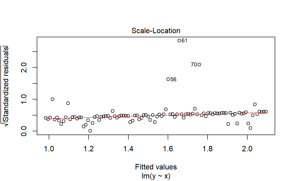

plot(lm(y ~ x), which=3)

R-squared is very low and our residuals vs. fitted plot reveals outliers and non-constant variance. A common fix for this is to log transform the data. Let’s try that and see what happens:

plot(lm(log(y)~x),which = 3)

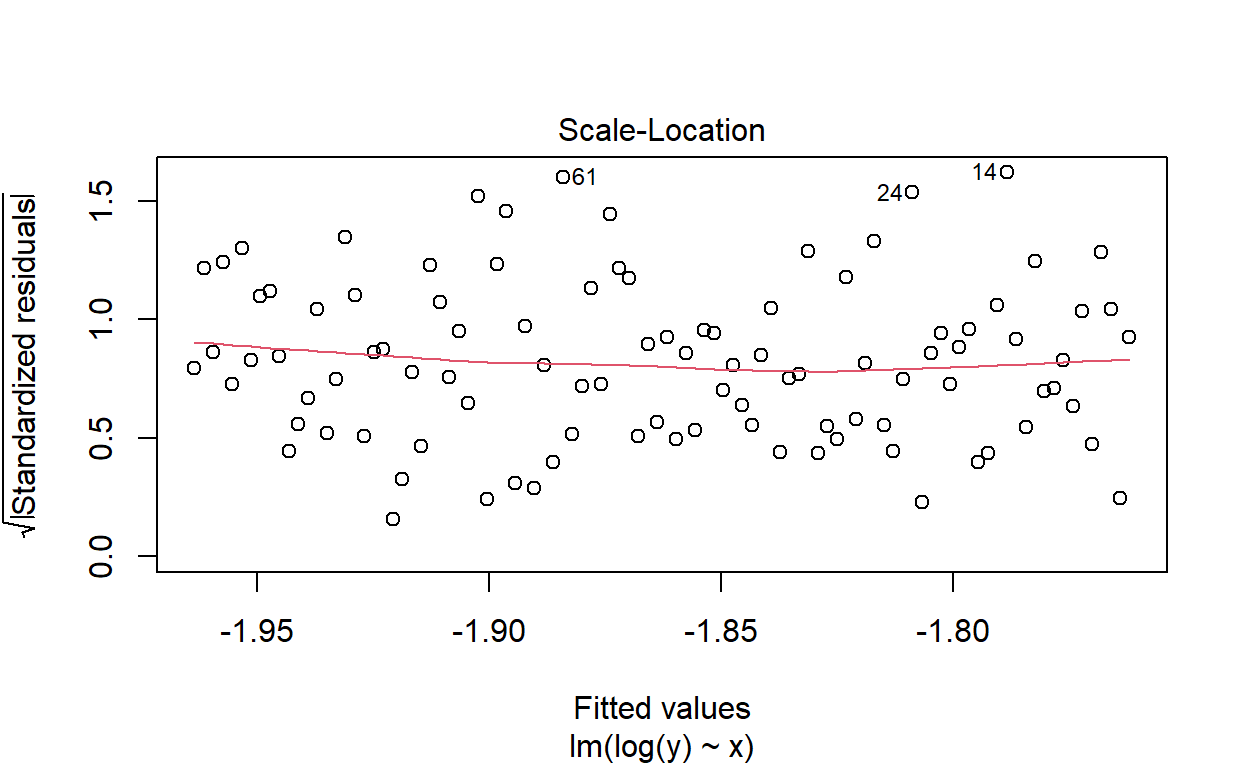
The diagnostic plot looks much better. Our assumption of constant variance appears to be met. But look at the R-squared:

summary(lm(log(y)~x))$r.squared

[1] 0.0006921086

It’s even lower! This is an extreme case and it doesn’t always happen like this. In fact, a log transformation will usually produce an increase in R-squared. But as just demonstrated, assumptions that are better fulfilled don’t always lead to higher R-squared.

It is very common to say that R-squared is “the fraction of variance explained” by the regression. \[Yet\] if we regressed X on Y, we’d get exactly the same R-squared. This in itself should be enough to show that a high R-squared says nothing about explaining one variable by another.

This is the easiest statement to demonstrate:

x <- seq(1,10,length.out = 100)
y <- 2 + 1.2*x + rnorm(100,0,sd = 2)
summary(lm(y ~ x))$r.squared

[1] 0.737738

summary(lm(x ~ y))$r.squared

[1] 0.737738

Does x explain y, or does y explain x? Are we saying “explain” to dance around the word “cause”? In a simple scenario with two variables such as this, R-squared is simply the square of the correlation between x and y:

all.equal(cor(x,y)^2, summary(lm(x ~ y))$r.squared, summary(lm(y ~ x))$r.squared)

[1] TRUE

Let’s recap:

R-squared does not measure goodness of fit.
R-squared does not measure predictive error.
R-squared does not necessarily increase when assumptions are better satisfied.
R-squared does not measure how one variable explains another.

https://data.library.virginia.edu/is-r-squared-useless/↩︎

Rsquared Bad

Time to blow RSquared up1 💥

Time to blow RSquared up¹ 💥