Module 4 Lagniappe

The extra info for module 4 is online.

Filtering Joins

Filtering joins match observations in the same way as mutating joins, but affect the observations, not the variables. There are two types:

• semi_join(x, y) keeps all observations in x that have a match in y.

• anti_join(x, y) drops all observations in x that have a match in y.

Semi-joins are useful for matching filtered summary tables back to the original rows.

Graphically, a semi-join looks like this:

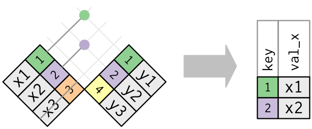
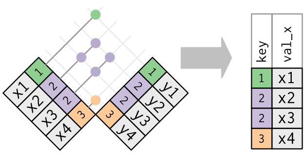
Only the existence of a match is important; it doesn’t matter which observation is matched. This means that filtering joins never duplicate rows like mutating joins do:

The inverse of a semi-join is an anti-join. An anti-join keeps the rows that don’t have a match:

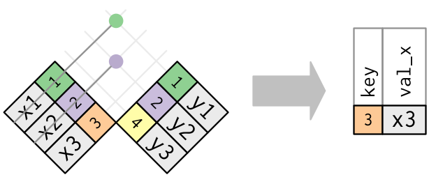
Anti-joins are useful for diagnosing join mismatches.

Set Operations

The final type of two-table verb are the set operations. Generally, I use these the least frequently, but they are occasionally useful when you want to break a single complex filter into simpler pieces. All these operations work with a complete row, comparing the values of every variable. These expect the x and y inputs to have the same variables, and treat the observations like sets:

• intersect(x, y): return only observations in both x and y.

• union(x, y): return unique observations in x and y.

• setdiff(x, y): return observations in x, but not in y.

Given this simple data:

library(tidyverse)

df1 <- tribble(
  ~x, ~y,
   1,  1,
   2,  1
)
df2 <- tribble(
  ~x, ~y,
   1,  1,
   1,  2
)

The four possibilities are:

intersect(df1, df2)

# A tibble: 1 x 2
      x     y
  <dbl> <dbl>
1     1     1

#> # A tibble: 1 x 2
#>       x     y
#>   <dbl> <dbl>
#> 1     1     1

# Note that we get 3 rows, not 4
union(df1, df2)

# A tibble: 3 x 2
      x     y
  <dbl> <dbl>
1     1     1
2     2     1
3     1     2

#> # A tibble: 3 x 2
#>       x     y
#>   <dbl> <dbl>
#> 1     1     1
#> 2     2     1
#> 3     1     2

setdiff(df1, df2)

# A tibble: 1 x 2
      x     y
  <dbl> <dbl>
1     2     1

#> # A tibble: 1 x 2
#>       x     y
#>   <dbl> <dbl>
#> 1     2     1

setdiff(df2, df1)

# A tibble: 1 x 2
      x     y
  <dbl> <dbl>
1     1     2

#> # A tibble: 1 x 2
#>       x     y
#>   <dbl> <dbl>
#> 1     1     2

---

This is an important property of what’s known as normal forms of data. The process of decomposing data frames into less redundant tables without losing information is called normalization. More information is available on Wikipedia.

Both dplyr and SQL we mentioned in the introduction of this chapter use such normal forms. Given that they share such commonalities, once you learn either of these two tools, you can learn the other very easily.

Data Transformation with dplyr cheatsheet.

Another useful function is rename(), which as you may have guessed changes the name of variables.

We can also return the top n values of a variable using the top_n() function.