PWC Excel Case Study
Information not discussed in class
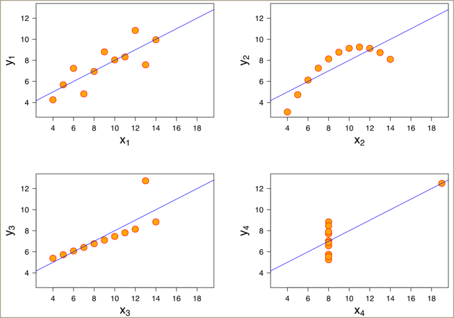
“Anscombe’s quartet”
| \(\color{red}{\text{Property}}\) | \(\color{red}{\text{Value}}\) | \(\color{red}{\text{Accuracy}}\) |
|---|---|---|
| Mean of x | 9 | exact |
| Sample variance of x | 11 | exact |
| Mean of y | 7.5 | 2 decimal places |
| Sample variance of y | 4.125 | plus/minus 0.003 |
| Correlation between x and y | 0.816 | 3 decimal places |
| Linear regression line | y = 3.00 + 0.500x | 2-3 decimal places |
Visualizing the quartet
Index function
- An alternative approach that offers greater flexibility is to use a combination of the INDEX and MATCH functions.
- INDEX returns the value at a particular position (index) in a range
Syntax
=INDEX ( \(\color{red}{\text{range of values}}\), \(\color{maroon}{\text{row number}}\), \(\color{green}{\text{column number (optional)}}\) )
Example
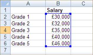
=INDEX (\(\color{red}{\text{B2:B6}}\), \(\color{maroon}{\text{4}}\))
Returns a value of 40,000, because 40,000 is in the fourth row of the range.
Match
- MATCH is used to find which row or column in a list contains a particular value
- Typically the match type should be set to zero for an exact match
Syntax
=MATCH ( \(\color{red}{\text{value to find}}\), \(\color{maroon}{\text{range to search}}\), \(\color{green}{\text{match type (optional)}}\) )
Example
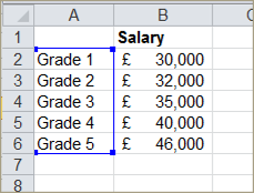
=MATCH (\(\color{red}{\text{"Grade 3"}}\), \(\color{maroon}{\text{A2:A6}}\), \(\color{green}{\text{0}}\))
Returns a value of 3, because ‘Grade 3’ is in the third cell of the range
Index/Match
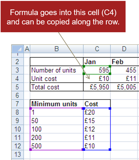
Example: Find the unit cost based on the number of units
First we use a MATCH function to find the appropriate row based on the (approximate) number of units:
- =MATCH(\(\color{red}{\text{C3}}\),$B$8:$B$12,\(\color{maroon}{\text{1}}\))
Then we use an INDEX function to retrieve the cost value contained in this row:
- =INDEX($C$8:$C$12, row number goes here )
These combine to make an overall formula:
- =INDEX($C$8:$C$12,MATCH(\(\color{red}{\text{C3}}\),$B$8:$B$12,\(\color{maroon}{\text{1}}\)))
In this example, the number of units is 595, and the formula returns $10.
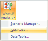
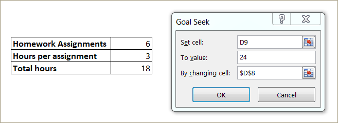
Optimization
Goalseek provides a way to solve simple equations
- Set a cell to a value
- Change another cell to produce the set value
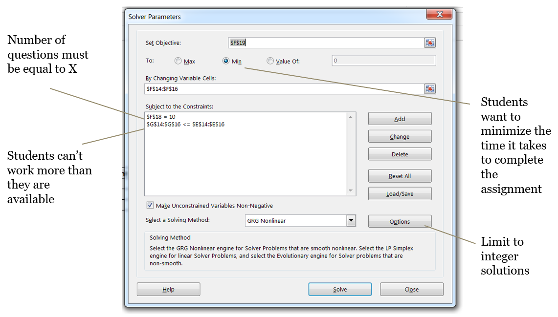
Solver provides more powerful and scalable optimization for systems of equations
Solver - Objective and constraints